Too Wide or Not Too Wide | That is the ClickHouse® Question

ClickHouse users often ask, “How many columns are too many? Can I have a table with 100 columns? 1000 columns? 5000 columns?” In truth there is no exact answer. We used to answer “don’t guess, but test.” So we decided to create an extreme example with 10 thousand (!) columns and put it to the test! In fact, we were not sure ourselves what to expect. However, it worked quite well but required some configuration tweaks and enough memory. We also ran into several important trade-offs. Intrigued? Read the rest of the article.
If you love ClickHouse®, Altinity can simplify your experience with our fully managed service in your cloud (BYOC) or our cloud and 24/7 expert support. Learn more.
Use Case
Consider a monitoring application that collects metrics from various device types. Every device type may have a unique set of different metrics. When stored in a single table that may result in hundreds or even thousands of metrics. As explained in our article “Handling Variable Time Series Efficiently in ClickHouse”, there are a number of approaches that one can take. The most efficient way is to keep every metric in a separate column. That works best when metrics are known in advance. For variable time series, e.g. when new device types are added dynamically, other approaches can be used, such as storing metrics in key-value arrays or map-like structures.
However, adding a new column to ClickHouse is very inexpensive, and we have seen a common practice where ClickHouse users are adding new columns on a regular basis. For example, when a new metric appears, or in order to materialize most frequently used metrics stored in raw JSON or arrays. That can result in very wide tables with hundreds or thousands of columns.
Creating 10K column table
Creating a table with a CREATE TABLE statement is easy when the number of columns is not too big. However, if we need thousands of columns some automation would be very much welcomed, otherwise one risks spending his day typing column names. For the purpose of our test let’s generate the table definition using, of course, an SQL statement:
WITH cols as (SELECT 'col' || toString(number) as col_name, 'Int32' as col_type from numbers(10000))
SELECT
'CREATE TABLE events_wide (
timestamp DateTime,
device_id String,
' || arrayStringConcat(arrayMap( (k, t) -> k || ' ' || t, groupArray(col_name), groupArray(col_type)), ',\n')
|| '
)
ENGINE = MergeTree
PARTITION BY toYYYYMMDD(timestamp)
ORDER BY (device_id, timestamp)
' as create_table
FROM cols
FORMAT TSVRaw
Here we use ClickHouse number generator to produce a dataset with 10K rows that define columns and datatypes. We then convert rows to column definitions using routine array magic. Format ‘TSVRaw’ is important – it keeps all line ends and quotes characters in place.
The result is a huge 10K+ lines CREATE TABLE statement:
CREATE TABLE events_wide (
timestamp DateTime,
device_id String,
col0 Int32,
col1 Int32,
col2 Int32,
...
col9999 Int32
)
ENGINE = MergeTree
PARTITION BY toYYYYMMDD(timestamp)
ORDER BY (device_id, timestamp)
In order to load the table definition to ClickHouse we can copy/paste the giant DDL statement, or use pipe:
clickhouse-local --query="WITH cols as (SELECT 'col' || toString(number) as col_name, 'Int32' as col_type from numbers(10000))
SELECT
'CREATE TABLE events_wide (
timestamp DateTime,
device_id String,
' || arrayStringConcat(arrayMap( (k, t) -> k || ' ' || t, groupArray(col_name), groupArray(col_type)), ',\n')
|| '
)
ENGINE = MergeTree
PARTITION BY toYYYYMMDD(timestamp)
ORDER BY (device_id, timestamp)
' as create_table
FROM cols
FORMAT TSVRaw" | clickhouse-client -h <my-server> --user=<my-user> --password
Now we’ve got a 10K columns table, what’s next? Let’s also create a table that would store all metrics in a Map for comparison:
CREATE TABLE events_map (
 timestamp DateTime,
 device_id String,
 metrics Map(LowCardinality(String), Int32)
)
ENGINE = MergeTree
PARTITION BY toYYYYMMDD(timestamp)
ORDER BY (device_id, timestamp)
Once we’ve created tables, we need to load the test data.
Inserting into a 10K column table
There are multiple ways to load data into ClickHouse. We will use meta programming one more time here in order to generate the giant INSERT statement. It will allow us to probe some more ClickHouse limits:
WITH cols as (SELECT 'col' || toString(number) as col_name, 'Int32' as col_type from numbers(10000)),
     1000 as devices,
     1000000 as rows
SELECT
'
INSERT INTO events_wide
SELECT
now() timestamp,
toString(rand(0)%' || toString(devices) || ') device_id,
' || arrayStringConcat( arrayMap( c -> 'number as ' || c, groupArray(col_name)),',\n')
||
'
FROM numbers(' || toString(rows) || ')'
FROM cols
FORMAT TSVRaw
The script has 3 variables in ‘WITH’ section that can be altered:
- ‘cols’ generates the list of columns, as we did for
CREATE TABLE - ‘devices’ specifies the number of unique devices_ids
- ‘rows’ specifies number of rows to be inserted
In every row all columns get the same value, but that’s ok for the purpose of this research.
The generated INSERT statement can be stored in a file, so we can quickly re-run it and make small adjustments. It will look like this:
INSERT INTO events_wide
SELECT
now() timestamp,
toString(rand(0)%1000) device_id,
number as col0,
number as col1,
number as col2,
...
number as col9999
FROM numbers(1000000)
Once we generate the INSERT statement and try to execute it we get the to the first bump:
Max query size exceeded: '9114'. (SYNTAX_ERROR)
Our INSERT statement size is 287K, which is above the default ClickHouse limit (256K). We need to increase the max_query_size setting. It can be added to clickhouse-client as a parameter, for example:
cat q.sql | clickhouse-client –max_query_size=1000000
Let’s set it to 1M and try running the loading script one more time.
AST is too big. Maximum: 50000. (TOO_BIG_AST)
Another bump! Now ClickHouse parser complains that the query is too complex. max_ast_elements needs to be increased, the default is 50K. Let’s increase it as well. And… we now bump into a memory problem:
Memory limit (total) exceeded: would use 12.60 GiB (attempt to allocate chunk of 4194320 bytes)
Initially we used a small machine with 4vCPU and 16GB of RAM for these tests and it does not seem to be enough for 10K columns. ClickHouse allocates a 2 MB buffer for every column, so for 10K columns it probably requires more than 20GB of RAM. Let’s re-scale the cluster up to the bigger node size and prove we can load the data if there is more RAM. In Altinity.Cloud it takes just a few minutes to upgrade the node size, in order to try 16 vCPU / 64GB RAM server and get:
Memory limit (for query) exceeded: would use 53.11 GiB (attempt to allocate chunk of 8000256 bytes), maximum: 53.10 GiB. (MEMORY_LIMIT_EXCEEDED)
Never give up! Let’s scale it to a 32 vCPU / 128GB instance.
That finally worked!
167 seconds and we are done – 1M rows were loaded into a 10K column table! We can now check the query_log and see that the peak memory usage was 64GB.
Is it possible to decrease the memory footprint? What if we enable compact parts for MergeTree table? Columns in a compact part are stored together in a single file (separate files for data and marks, to be accurate), and the offset of every column is stored as well. So it is still columnar, but instead of writing and reading separate files per column, ClickHouse seeks in a small number of files. With a smaller number of files we would expect better insert performance and less memory consumption.
In order to enable compact parts we need to set min_bytes_for_wide_part and min_rows_for_wide_part to some bigger values. These are table level settings, and can be modified with an ALTER TABLE statement. For comparison purposes, however, we will create a new table:
CREATE TABLE events_compact as events_wide
ENGINE = MergeTree
PARTITION BY toYYYYMMDD(timestamp)
ORDER BY (device_id, timestamp)
SETTINGS
min_bytes_for_wide_part=1048576000,
min_rows_for_wide_part=1048576;
So we are setting 100MB and 1M rows limits for compact parts this way.
Let’s run the same insert statement as we did earlier, but to the altered table. Quite surprisingly, inserting into events_compact table took 25% more time and RAM: 214s and 82GB!
Finally, let’s load the data into the events_map table using the following SQL. We do not need meta-programming since we can construct map during query execution:
INSERT INTO events_map
WITH arrayMap( n -> 'col' || toString(n), range(10000)) as cols
SELECT
  now() timestamp,
  toString(rand(0)%1000) device_id,
  arrayMap( c -> (c,number), cols)
FROM numbers(1000000)
This query constructs an array of tuples [('col0', number), ... , ('col9999', number)] for every row that is converted into a Map data on INSERT. This ran out of RAM again, so we had to do yet another trick: reduce the block size. Here’s how:
SELECT ... SETTINGS max_block_size=100000Loading into the events_map table was ridiculously slow. It took 13 mins with 45GB peak memory usage even with a reduced block size. However, the problem in this case was not INSERT but the SELECT part of the query. Unlike queries to wide and compact tables, here we had to manipulate with 10K element arrays for every row. It is slow and memory intensive. We have tried a number of experiments in order to optimize this query but could not get better results even when inserting a constant or loading prepared data from the file! It looks like the main overhead is in handling huge arrays.
Since 100K row blocks helped to reduce the memory footprint for events_map, let’s try the same with wide and compact tables. Results were quite interesting: memory usage has been reduced significantly for the compact parts table, but stayed almost the same for the wide table. Here is a summary:
| Table Name | Load 1M rows | RAM 1M rows | Load 10x100K rows | RAM 10x100K rows |
| events_wide | 167s | 64GB | 156s | 50GB |
| events_compact | 212s | 82GB | 157s | 9.3GB |
| events_map | | | | | 780s | 45GB |
Now let’s take a look into parts for all tables:
select table, part_type, count(), sum(rows), sum(bytes_on_disk) bytes_on_disk, sum(data_uncompressed_bytes) uncompressed from system.parts where table like 'events_%' group by table, part_type order by table

┌─table──────────┬─part_type─┬─count()─┬─sum(rows)─┬─bytes_on_disk─┬─uncompressed─┐
│ events_compact │ Compact   │      10 │   1000000 │   41794344282 │  40007890218 │
│ events_map     │ Wide      │       2 │   1000000 │     843832859 │  60463651504 │
│ events_wide    │ Wide      │      10 │   1000000 │   41089353783 │  40007889959 │
└───────────────┴───────────┴─────────┴───────────┴───────────────┴───────────────┘
Uncompressed data size in events_map table is bigger because column names are now stored on every row in the map, but compressed size is dramatically smaller – thanks to test data with a lot of repetitions that can be compressed much better in a row-like format.
Another potential caveat of wide tables is background merge performance. Let’s also take a look at merge performance running OPTIMIZE TABLE FINAL statements for respective tables.
| Table | Merge time |
| events_wide | 410s |
| events_compact | 2500s |
| events_map | 1060s |
First of all, we can see that merge is very slow! It takes more time to merge 10M wide rows than to load them initially. Merge performance for a compact parts table is just terrible! Even though we saved on RAM when inserted into events_compact, we paid later with a very heavy load on merges.
Loading hints summary:
- Increase
max_query_sizesetting to 1M, this is required to handle giant SQLs - Increase
max_ast_elementssetting to 256K, this is required to handle giant SQLs as well - Have more than 64GB of RAM
- Decrease
max_block_sizeif there is not enough RAM. - Using compact parts may reduce RAM utilization but has other drawbacks, like slower inserts and very slow merges.
Querying 10K rows table
In order to test query performance we run following queries:
- Full scan query:
select count() from events_wide where not ignore(*)- Top 10 devices by some metric:
select device_id, max(col1234) col1234
  from events_wide
 group by device_id
order by col1234 desc limit 10- Multiple metrics for a single device grouped by time dimension:
select timestamp ts,
  avg(col111) col111, avg(col222) col222, avg(col333) col333, avg(col444) col444
  from events_wide
 where device_id = '555'
 group by ts
 order by ts
Queries to events_map table need to be slightly modified to use metrics['colXYZ'] instead of colXYZ.
Here is elapsed time and memory usage for queries:
| Table | Q1 | Q2 | Q3 |
| events_wide | 126s / 47 GB | 0.052s / 58 MB | 0.047s / 13 MB |
| events_compact | 160s / 40 GB | 0.046s / 59 MB | 0.072s / 10 MB |
| events_map | 4.5s / 255 MB | 8.8s / 9 GB | 0.170s / 102 MB |
10K column tables are expectedly slow and memory hungry when all columns are selected but blazingly fast for queries touching subsets of columns.
Map table was much faster on a full scan, performed ok on a single device but was slow when scanning a metric across all devices, since ClickHouse had to read and scan the huge Map column every time.
In general, query performance for typical monitoring queries Q2 and Q3 is not affected by a number of columns – thanks to ClickHouse columnar data format. Only events_map table, that is essentially a row format, feels the extra load.
Shrinking to 1000 columns
When loading 10,000 columns we have faced a few challenges. What if we reduce the number of columns to only one thousand? Let’s test!
Same queries to create schema and data can be used as above, just change the number of columns to be 1000 instead of 10,000. With 1000 columns we did not have to apply any special settings, system defaults worked just fine, and we could load 1M rows in one block.
With 1000 columns load performance was exactly 10 times faster compared to 10 thousand, and merge was fast as well:
| Table Name | Load 1M rows | RAM 1M rows | Merge 1M rows |
| events_wide | 12s | 6.5GB | 11s |
| events_compact | 13s | 8.2GB | 9.3s |
| events_map | 74s | 36GB | 4.1s |
ClickHouse default insert block size is 1048545. So we can assume that with defaults ClickHouse will consume the same amount of RAM for bigger inserts as well. The memory usage for events_map table is still high, though. Handling huge maps and arrays is memory intensive. That leads us to the next section.
What about sparse wide tables?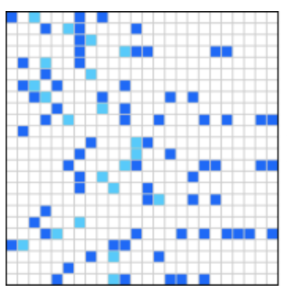

In real applications, one device will never produce 10K metrics. Usually, one device type is responsible for 10-100 metrics. However, multiple device types may produce different sets of metrics. When stored in a single monitoring table it may result in wide tables as discussed in the section above. Those tables have to be sparse, since only a fraction of columns for every row would have data, and other columns would be nulls. Since we sort a table by device, and metrics for a single device are usually grouped together, the data distribution in the matrix is block-sparse.
Map table would be much more compact in this case, since it does not have to store nulls. It would be interesting to measure ClickHouse in this scenario as well, but that would make this article too long. Let us just show how a sparse map table would look like.
The script below generates 1M rows but for every device it only puts 100 metrics to the map out of 10K possible ones.
INSERT INTO events_map_sparse
SELECT
now() timestamp,
toString(rand(0)%1000 as did) device_id,
arrayMap( c -> ('col' || toString(c), number), range(did*10, did*10 + 100))
FROM numbers(1000000)
SETTINGS function_range_max_elements_in_block=1000000000
This takes only 8s to load in a single block! The data size is reduced 100 times compared to a full 10K values:
┌─table─────────────┬─part_type─┬─count()─┬─sum(rows)─┬─bytes_on_disk─┬─uncompressed─┐
│ events_map        │ Wide      │       2 │   1000000 │     843832859 │  60463651504 │
│ events_map_sparse │ Wide      │       1 │   1000000 │       8014874 │    601591449 │
└──────────────────┴───────────┴─────────┴───────────┴───────────────┴───────────────┘
Queries are proportionally faster as well.
Wide table or multiple tables
Another design alternative is to use multiple tables, one per device type. Thus, instead of 10K columns wide table, we can have 100 tables with 100 columns each. This may seem plausible at the first glance, but it is just another trade off. While inserting to such “ordinary” tables is easy, there are 100 times more inserts. Also managing a lot of tables may be complicated. The total overhead on merges will be higher for 100 tables, compared to one wide table. Ingestion pipeline looks more complex as well. Application layers need to know how to route queries into appropriate tables and so on. Certainly, those are not blockers at all, and may work for users who are ready to carry management overhead on their own.
Conclusion
Going to extremes is fun but tough. Very wide tables in ClickHouse are not an exception. They work but may require extra tuning and a lot of RAM when inserting the data and performing maintenance operations, like merges or mutations, for example. In return users get outstanding ClickHouse query performance: for typical analytical queries 10 column table and 10 thousand column tables are not different. When handling thousands of columns is not desirable, the Map data type can be used. It can provide a good compromise between convenience and performance, especially for sparse tables, when only a fraction of the 10K columns is used in a row.
Answering to the question posed at the beginning of the article: 10,000 columns seem pretty demanding, but 1000 work just fine out of the box. Using sparse tables makes it easier as well.
The power of ClickHouse is in its flexibility. Users are not bound to use a single schema design. There are multiple options available. Understanding the pros and cons of different approaches is important for every ClickHouse user. Understanding grows from experience. Try it out and stay tuned!
ClickHouse® is a registered trademark of ClickHouse, Inc.; Altinity is not affiliated with or associated with ClickHouse, Inc.