Battle of the Views – ClickHouse Window View vs Live View

ClickHouse added experimental Window Views starting from 21.12. Window Views aggregate data over a period of time, then automatically post at the end of the period. They add another exciting tool for stream processing and analytics to ClickHouse’s toolbox while expanding its collection of view tables. In general, the concepts behind Window View can also be found in other systems, such as Azure Stream Analytics, Kafka Streams, and Apache Spark among others.

Window Views follow the addition of experimental Live View tables added in 19.14.3.3. In this article, we will look at both of them to find the differences and similarities between the two. Let’s get a better view on these two different views!

General Applications

Window View allows you to compute aggregates over time windows, as records arrive in real-time into the database, and provides similar functionality that is typically found in other stream processing systems.

Typical applications include keeping track of statistics, such as calculated average values over the last 5 minutes or a 1 hour window, which can be used to detect anomalies in a data stream while grouping data by time into one or more active time windows.

On the other hand, Live View is not specialized for time window processing and is meant to provide real-time results for common queries without the need to necessarily group arriving records by time. 

Some typical applications, as pointed out in the documentation, include providing real-time push notifications for query result changes to avoid polling, caching the results of the most frequently used queries, detecting table changes and triggering follow-up queries, as well as real-time monitoring of system table metrics using periodic refresh.

Overview

In order for us to examine both Window View and Live View, we must first understand how they work.

As we have blogged about Live View before, please see our previous articles for more detailed information Making Data Come to Life with ClickHouse Live View Tables, Taking a Closer Look at ClickHouse Live View Tables, Using Live View Tables with a Real Dataset, and, finally, Real-time Moving Average with ClickHouse Live Views.

However, we haven’t blogged about Window View before, so a quick introduction is necessary. For more details, check out the Window View documentation.

Window View

Window View is designed to work with Time Window Functions, in particular Tumble and Hop. These time window functions are used to group records together over which an aggregate function can be applied. The time reference can either be set to the current time, as provided by the now() function, or as a table column.

To better understand Time Window Functions, we can visualise them as follows:

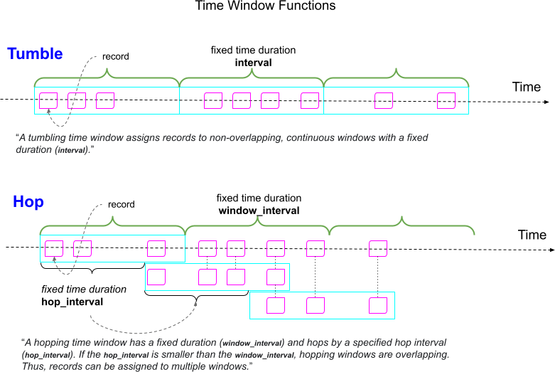
For processed results, the Window View can either push to a specified table or push real-time updates using the WATCH query.

Live View

On the other hand, Live View, is not tied to any group by function. Instead, it allows you to provide streaming query results for queries where the result of the query can be computed by applying the same query on the current data and the new data separately, and merging the results of the two to compute the final result. Live View query processing can be visualised as follows:

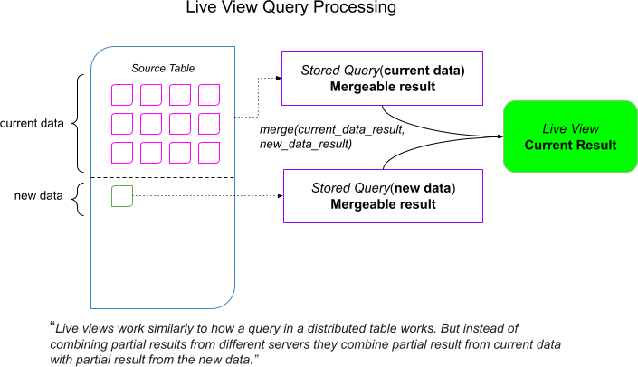
Live View can output the computed result by SELECTing from it, or it can push real-time updates using the WATCH query.

Comparison In Action

Let’s use the following source table to see how Window View and Live View work in action. We will use ClickHouse 22.3.6.5 for our examples.

CREATE TABLE data (`id` UInt64, `timestamp` DateTime) ENGINE = MergeTree() ORDER BY tuple();

Because both features are experimental, we need to ‘set’ the corresponding settings to make them available.

set allow_experimental_live_view = 1
set allow_experimental_window_view = 1

Example: Counting Number Of Events Per Interval

The default example provided in the Window View documentation shows an example of how we can use Window View to count the number of events, per 10 seconds, using the live data that comes into our data table. In this case, the tumble() time window function is ideal to provide non-overlapping fixed interval time windows. The tumbleStart() function can be used to get the front edge of the time window.

CREATE WINDOW VIEW wv AS
SELECT
    count(id),
    tumbleStart(w_id) AS window_start
FROM data
GROUP BY tumble(timestamp, toIntervalSecond('10')) AS w_id

Let’s try to do something similar using a Live View. Our first attempt uses the following query:

CREATE LIVE VIEW lv AS
SELECT
    count(id),
    toStartOfInterval(timestamp, toIntervalSecond(10)) AS window_start
FROM data
GROUP BY window_start

Now let’s start WATCHing both views while inserting records into the source table and observing the results. We will need three active ClickHouse client sessions, as two of them will be used to run WATCH queries and the third will be used to perform INSERTs.

Open clickhouse-client1 and execute:

WATCH wv

Then, open clickhouse-client2 and execute:

WATCH lv

You should see that both WATCH queries are stuck without any output, as the WATCH query blocks to output an infinite stream of results until it is aborted if the LIMIT clause is not specified. There is no data in our source data table and, therefore, no output yet.

Next, let’s insert some rows into the source data table in clickhouse-client3:

INSERT INTO data VALUES(1,now())

We can immediately observe that WATCH lv query provides immediate output while WATCH wv output is delayed until the time window closes.

Both outputs after 10 sec are the following.

WATCH lv

┌─count(id)─┬────────window_start─┬─_version─┐
│         1 │ 2022-06-28 15:23:20 │        2 │
└───────────┴─────────────────────┴──────────┘

WATCH wv

┌─count(id)─┬────────window_start─┐
│         1 │ 2022-06-28 15:23:20 │
└───────────┴─────────────────────┘

Disregarding the _version column in the WATCH lv output, we see that the results are the same.

Now let’s do exactly the same INSERT one more time. The new result for both is as follows:

INSERT INTO data VALUES(1,now())

WATCH lv

┌─count(id)─┬────────window_start─┬─_version─┐
│         1 │ 2022-06-28 15:27:00 │        3 │
│         1 │ 2022-06-28 15:23:20 │        3 │
└───────────┴─────────────────────┴──────────┘

WATCH wv

┌─count(id)─┬────────window_start─┐
│         1 │ 2022-06-28 15:27:00 │
└───────────┴─────────────────────┘

As we can see, the Live View’s second result contains data for both time intervals, while the result of the Window View only shows the result of the latest time window.

Let’s confirm this behaviour by doing two more identical INSERTs as before, one after another:

INSERT INTO data VALUES(1,now())
INSERT INTO data VALUES(1,now())

WATCH lv

┌─count(id)─┬────────window_start─┬─_version─┐
│         2 │ 2022-06-28 15:30:00 │        5 │
│         1 │ 2022-06-28 15:27:00 │        5 │
│         1 │ 2022-06-28 15:23:20 │        5 │
└───────────┴─────────────────────┴──────────┘

WATCH wv

┌─count(id)─┬────────window_start─┐
│         2 │ 2022-06-28 15:30:00 │
└───────────┴─────────────────────┘

The results are as expected. The Live View keeps accumulating results for all the time intervals, while the Window View with the tumble() time window function only outputs the result for the last closed time window.

Let’s abort WATCH lv query and DROP the current Live View, and replace it with the following view that tries to mimic the behaviour of the Window View.

CREATE LIVE VIEW lv AS
SELECT
    count(id),
    toStartOfInterval(timestamp, toIntervalSecond(10)) AS window_start
FROM data
GROUP BY window_start
ORDER BY window_start DESC
LIMIT 1

Now let’s restart the WATCH lv query in clickhouse-client2:

WATCH lv

We can see that the WATCH lv now returns the same data as WATCH wv.

┌─count(id)─┬────────window_start─┬─_version─┐
│         2 │ 2022-06-28 15:30:00 │        1 │
└───────────┴─────────────────────┴──────────┘

Let’s do two more INSERTs:

INSERT INTO data VALUES(1,now())
INSERT INTO data VALUES(1,now())

We can see that the last result for the Window View and the Live View match.

WATCH wv

┌─count(id)─┬────────window_start─┐
│         2 │ 2022-06-28 15:42:50 │
└───────────┴─────────────────────┘

WATCH lv

┌─count(id)─┬────────window_start─┬─_version─┐
│         2 │ 2022-06-28 15:42:50 │        3 │
└───────────┴─────────────────────┴──────────┘

Using Time Window Functions In Live View

It’s time to have some fun and use the tumble() and tumbleStart() functions in Live View instead of Window View:

CREATE LIVE VIEW lv AS
SELECT
    count(id),
    tumble(timestamp, toIntervalSecond('10')) AS w_id,
    tumbleStart(w_id) AS window_start
FROM data
GROUP BY w_id

Now, if we do WATCH lv, we get:

┌─count(id)─┬─w_id──────────────────────────────────────────┬────────window_start─┬─_version─┐
│         2 │ ('2022-06-28 15:30:00','2022-06-28 15:30:10') │ 2022-06-28 15:30:00 │        1 │
│         1 │ ('2022-06-28 15:27:00','2022-06-28 15:27:10') │ 2022-06-28 15:27:00 │        1 │
│         2 │ ('2022-06-28 15:42:50','2022-06-28 15:43:00') │ 2022-06-28 15:42:50 │        1 │
│         1 │ ('2022-06-28 15:23:20','2022-06-28 15:23:30') │ 2022-06-28 15:23:20 │        1 │
└───────────┴───────────────────────────────────────────────┴─────────────────────┴──────────┘

This shows that Live View can be used with tumble() and tumbleStart() functions.

Let’s modify our Live View query as before to match the output of Window View:

CREATE LIVE VIEW lv AS
SELECT
    count(id),
    tumble(timestamp, toIntervalSecond('10')) AS w_id,
    tumbleStart(w_id) AS window_start
FROM data
GROUP BY w_id
ORDER BY w_id DESC
LIMIT 1

Now, we get the following for WATCH lv:

┌─count(id)─┬─w_id──────────────────────────────────────────┬────────window_start─┬─_version─┐
│         2 │ ('2022-06-28 15:42:50','2022-06-28 15:43:00') │ 2022-06-28 15:42:50 │        1 │
└───────────┴───────────────────────────────────────────────┴─────────────────────┴──────────┘

Again, let’s perform a couple of new INSERTs to compare the results of Window View and Live View:

INSERT INTO data VALUES(1,now())
INSERT INTO data VALUES(1,now())

Note that, depending on query timing, different inserts can go into different time windows. If that happens, just try your INSERTs again.

WATCH wv

┌─count(id)─┬────────window_start─┐
│         2 │ 2022-06-28 15:53:00 │
└───────────┴─────────────────────┘

WATCH lv

┌─count(id)─┬─w_id──────────────────────────────────────────┬────────window_start─┬─_version─┐
│         1 │ ('2022-06-28 15:53:00','2022-06-28 15:53:10') │ 2022-06-28 15:53:00 │        4 │
└───────────┴───────────────────────────────────────────────┴─────────────────────┴──────────┘
┌─count(id)─┬─w_id──────────────────────────────────────────┬────────window_start─┬─_version─┐
│         2 │ ('2022-06-28 15:53:00','2022-06-28 15:53:10') │ 2022-06-28 15:53:00 │        5 │
└───────────┴───────────────────────────────────────────────┴─────────────────────┴──────────┘

After 10 sec passes, Window View closes the time window, and the results of Live View and Window View are the same. However, if you pay attention, you will see that the Live View provides immediate results for the current time window, as it does not wait for the time window to close.

When Window View and Live View Results Will Differ

So far, we have seen that we can make Live View behave very close to Window View. However, this is only because we used a table column for the time attribute to the tumble() time window function. When we try to use the now() function instead, the results from Live View will not be what you expect. You can see this if we drop the previous tables and create new ones as follows:

CREATE WINDOW VIEW wv AS
SELECT
    count(id),
    tumbleStart(w_id) AS window_start
FROM data
GROUP BY tumble(now(), toIntervalSecond('10')) AS w_id

CREATE LIVE VIEW lv AS
SELECT
    count(id),
    tumble(now(), toIntervalSecond('10')) AS w_id,
    tumbleStart(w_id) AS window_start
FROM data
GROUP BY w_id
ORDER BY w_id DESC
LIMIT 1

If you execute WATCH lv, you will see something like this:

WATCH lv

┌─count(id)─┬─w_id──────────────────────────────────────────┬────────window_start─┬─_version─┐
│        10 │ ('2022-06-28 16:34:50','2022-06-28 16:35:00') │ 2022-06-28 16:34:50 │        1 │
└───────────┴───────────────────────────────────────────────┴─────────────────────┴──────────┘

The WATCH wv will not provide output until you do an INSERT. If you try to do an INSERT, the Live View keeps assigning records to the same time window bucket, as the now() function is not re-evaluated in Live View when new data arrives but stays fixed, while the Window View properly creates time windows based on the current value of now() as expected.

When Live View Must Be Used Instead Of Window View

It is also useful to know when Live View must be used and Window View is not an option. Let’s see an example where we try to create a Window View that does not include the GROUP BY clause, which causes an error:

CREATE WINDOW VIEW wv AS
SELECT count(id)
FROM data

Received exception from server (version 22.3.6):
Code: 80. DB::Exception: Received from localhost:9000. DB::Exception: GROUP BY query is required for WindowView. (INCORRECT_QUERY)

This shows that Window View is meant to be used only with the GROUP BY clause. We can also check if the Window View can be used with GROUP BY that does not use one of the two time window functions. Again, we get an error:

CREATE WINDOW VIEW wv AS
SELECT count(id)
FROM data
GROUP BY toStartOfInterval(timestamp, toIntervalSecond(10))

Received exception from server (version 22.3.6):
Code: 80. DB::Exception: Received from localhost:9000. DB::Exception: TIME WINDOW FUNCTION is not specified for WindowView. (INCORRECT_QUERY)

Both of the above queries will work fine for Live View, as we can see below:

CREATE LIVE VIEW wv AS
SELECT count(id)
FROM data

WATCH lv

┌─count(id)─┬─w_id──────────────────────────────────────────┬────────window_start─┬─_version─┐
│        13 │ ('2022-06-28 16:37:10','2022-06-28 16:37:20') │ 2022-06-28 16:37:10 │        4 │
└───────────┴───────────────────────────────────────────────┴─────────────────────┴──────────┘

CREATE LIVE VIEW lv AS
SELECT count(id)
FROM data
GROUP BY toStartOfInterval(timestamp, toIntervalSecond(10))

WATCH lv

┌─count(id)─┬─_version─┐
│         2 │        1 │
│         1 │        1 │
│         1 │        1 │
│         2 │        1 │
│         1 │        1 │
│         2 │        1 │
│         2 │        1 │
│         1 │        1 │
│         1 │        1 │
└───────────┴──────────┘

Note that the Live View result in the last view grows with input and causes the server to run out of memory. Ensure you keep in mind that the result of the query should either be an aggregated value or be fixed using the LIMIT clause in the innermost query.

Other Differences

The other difference between Live View and Window View tables is that Window View stores its results in an inner table engine, which by default is AggregatingMergeTree if not specified explicitly using the INNER ENGINE clause when creating the view. Live View, on the other hand, currently stores all intermediate results only in memory, which can cause server memory issues when proper care is not taken.

Also, Window View can write its results to a dedicated table by specifying the TO clause, while Live View can only be used to SELECT and WATCH. A workaround for Live View is to use the INSERT INTO db.table WATCH [lv] statement to manually output results into a table.

Another big difference between Window View and Live View is that Window View supports defining windows based on processing time or event time, while also allowing control of how late events are processed. The event time is defined as the time emdedded in the arriving records and processing time is defined as the local machine’s time. In practical applications, using event time is more appropriate as it provides determinism, whereas using processing time does not.

Conclusion

While Window View and Live View tables have some similarities, they are best used for their intended purpose. It is also important to note that both of these features are still in an experimental mode and most likely will be modified in a backward incompatible mode as ClickHouse generalises support for streaming queries and stream analytics processing.

Nonetheless, these two features show the power of ClickHouse as an open-source project that allows third-party contributors to show how the core project can evolve to solve needs that were not initially anticipated by the core development team. These features are definitely worth a closer look, so keep WATCHing how Window View and Live View tables evolve in future ClickHouse releases.

If you would like to discuss these features in more detail or get assistance on any aspect of analytic applications on ClickHouse, you can contact us or join the AltinityDB slack channel. We look forward to hearing from you!