Managing geolocations with H3 indexing in ClickHouse®

If you love ClickHouse®, Altinity can simplify your experience with our fully managed service in your cloud (BYOC) or our cloud and 24/7 expert support. Learn more.
Imagine you’re managing a massive dataset of geospatial information—millions of cell towers scattered across the globe, each defined by nothing more than latitude and longitude. Running real-time queries on this kind of data can be slow, and drawing meaningful insights from it even slower. You can use PostGIS of course, but enter ClickHouse, famed for its lightning-fast columnar storage and query engine. Those great features now have a powerful upgrade: H3 indexing.
With H3, ClickHouse transforms geospatial data processing by breaking the world into a beautifully simple grid of hexagons. Suddenly, complex tasks like proximity searches, clustering, and geographic aggregations become efficient, scalable, and remarkably intuitive. Now, instead of wrestling with latitude and longitude coordinates, you can snap data into tidy hexagonal cells, instantly visualizing and querying the world in a way that feels natural and precise. ClickHouse with H3 doesn’t just handle geospatial data—it makes it sing, unlocking a new era of speed and simplicity in location-based analytics.
Geospatial data is crucial in a wide variety of industries, from mobile network analysis to fleet management, logistics, and location-based services. Efficiently querying, analyzing, and aggregating such data at scale can be challenging. That’s where tools like ClickHouse and H3 indexing come into play. In this article, we’ll explore how to leverage H3 indexing within ClickHouse to work with large geospatial datasets. We’ll use the OpenCellID dataset, which contains detailed data on cell towers across the globe.
Why use H3 Indexing?
But why H3 indexing? Originally developed by Uber as a spatial indexing system, it divides the world into hexagonal grids, offering better proximity calculations than traditional methods like latitude and longitude bounding boxes. H3’s hierarchical structure allows for more flexible and efficient geospatial analysis. Together, ClickHouse and H3 enable users to perform high-performance geospatial queries on large datasets with ease.

Figure 1: How H3 sees the world
The OpenCelliD dataset provides data about cell tower locations worldwide. Each record contains the latitude, longitude, and additional information about individual towers, such as their unique identifiers and network information. This dataset is used for:
- Mapping and visualizing mobile network coverage.
- Analyzing tower density and signal distribution in specific regions.
- Identifying tower proximity to other geospatial features or points of interest.
The dataset contains approximately 5 million rows, which is very easy to manage with ClickHouse. However, due to the unique nature of tower cell signal propagation, OpenCelliD is an ideal candidate for showcasing the capabilities of H3 indexing in ClickHouse. We’ll use the latest dataset from OpenCelliD. That gives us great sample data, and we don’t need to download it manually. We’ll just use the url() function to insert it in our schema. We’ll see how to do this later.
What is H3?
As we said earlier, H3 divides the Earth into a grid of hexagonal cells. Each cell has a unique identifier called an H3 index. This hierarchical structure allows for varying levels of resolution, making H3 a flexible and scalable solution for a wide range of geospatial queries and visualizations.
Each H3 cell can be subdivided into smaller hexagonal cells at higher resolutions. The system supports 16 resolutions, from level 0 (covering the entire Earth) to level 15 (which can drill down to a hexagonal area of roughly 0.9 m²). This hierarchical grid allows you to zoom in or out on specific regions while maintaining a consistent spatial relationship between cells.
| Resolution | Average Area per Hexagon (km²) | Use case |
| 0 | 4.35 Million | Entire world |
| 5 | 252 | Country or Regional aggregations |
| 9 | 0.10 | City block |
| 15 | 0.000000895 (0.895 m²) | High precision measurements |
For example:
- Resolution 0 is used when working with the entire Earth; the world is divided into 122 hexagons.
- Resolution 9 is often used in urban areas, providing hexagonal grids about the size of city blocks.
- Lower resolutions (like 5 or 6) are better for regional or country-level aggregation.
- For example, a hexagon for a resolution 15 h3 index will have these properties:
side: 0.55m
long diameter: 1.1m
short diameter: 0.95m
area: 0.8m2
perimeter: 3.3m
See the h3geo site for complete details on the exact area of hexagons at each level of resolution.
Why Use Hexagons?
Hexagons have several key advantages over grid shapes like squares or triangles, making them ideal for geospatial analysis:
- Equal Distance to Neighbors: Hexagonal cells have uniform edge lengths, meaning the distance from the center of one hexagon to its neighboring cells is consistent. This simplifies proximity searches and neighborhood queries.
- No Corner Adjacency: Unlike squares, which can touch at corners, hexagons are always adjacent along their edges, which avoids ambiguity in calculating neighbors or proximity. This makes them well-suited for efficient spatial clustering and aggregation.
- Efficient Coverage: Hexagons cover areas more naturally than squares, as they better approximate the shape of circular areas (which are common in real-world proximity calculations).
H3 and ClickHouse
H3 encodes latitude and longitude coordinates into unique hexagonal cells. ClickHouse provides a native H3 function set for working with geospatial data, allowing users to perform efficient spatial queries using hexagonal grids. The key functions include:
geoToH3(lon, lat, resolution): Converts longitude and latitude into an H3 index at the specified resolution. This allows for the encoding of geographic coordinates into hexagonal cells.h3ToGeo(h3_index): Converts an H3 index back into the center point (latitude and longitude) of the hexagonal cell.h3ToGeoBoundary(h3_index): Returns the polygon boundary of the hexagonal cell, providing the coordinates of the hexagon’s vertices.h3kRing(h3_index, k): Returns the set of H3 indexes within a givenkdistance (number of steps) from the target hexagon. This is useful for proximity searches within a specific radius.h3IsValid(h3_index): Checks whether an H3 index is valid, ensuring correct input during queries.
Why Use H3 with ClickHouse?
ClickHouse is known for its blazing-fast queries on large datasets. By combining ClickHouse with H3, we gain the following advantages:
- Spatial Query Efficiency: H3’s hierarchical structure and unique indexing mean you can quickly retrieve data for specific geographic areas. This is far more efficient than traditional latitude/longitude bounding boxes, especially when scaling to millions of points (such as cell towers).
- Simplified Queries: H3 reduces the complexity of geospatial queries. Instead of performing expensive distance calculations using latitude and longitude, you can use simple H3-based operations to determine proximity, clustering, or neighborhood queries.
- Scalability: H3 is designed to work well with massive datasets, just like ClickHouse. Together, they form a scalable solution for simple geospatial data analysis, making it easy to handle datasets as large as OpenCelliD or the TLC Trip Record Data for NYC taxis (which contains millions of indexes).
Don’t get me wrong, I also love PostGIS which is very powerful and optimized for many spatial operations and it is built on top of another great Open Source database, the row-oriented PostgreSQL. This makes PostGIS more suitable for moderately large datasets but less performant when scaling to very large datasets using ClickHouse and its column-oriented capabilities. While PostGIS supports analytical operations, its strength lies more in complex geospatial queries and detailed GIS operations like projections, advanced spatial joins or polygon operations, rather than large-scale, real-time analytics, like our case.
Comparison: H3 vs. Geohash Function Set
Geohash is a data format that represents square grid cells with strings of letters and numbers. H3 and Geohash both offer methods for spatial indexing, but they differ in structure and capabilities:
| Feature | H3 (Hexagonal) | Geohash (Square) |
| Shape | Hexagonal grid cells | Square grid cells |
| Resolution | 16 levels (hierarchical hexagon subdivisions) | Varies based on the number of geohash characters |
| Spatial Coverage | Uniform distance to neighboring cells (better for proximity queries) | Neighboring geohashes vary in size and shape |
| ClickHouse Functions | geoToH3(), h3ToGeoBoundary(), h3kRing() | geohashEncode(), geohashDecode(), geohashNeighbors() |
| Efficiency | Better for proximity-based operations due to consistent hexagonal edges | Sufficient for many cases, but square cells can lead to inaccuracies near borders |
| Common Use Cases | Clustering, proximity searches, geospatial joins | Geospatial data storage and simple spatial queries |
Key Differences:
- Shape and Distance: H3 uses hexagons, which offer uniform distance between neighboring cells, making it ideal for proximity searches. Geohash uses squares, which can lead to edge cases and inconsistencies near cell boundaries.
- Resolution: Both systems offer hierarchical structures, but H3’s hexagonal resolution is generally more consistent across geographic areas, whereas Geohash resolution may distort more near the poles.
- Functionality: H3 has more specialized functions for neighborhood searches and spatial aggregation, while Geohash is primarily focused on encoding and decoding geographic coordinates into alphanumeric strings.
In summary, H3 is generally better for advanced geospatial queries, particularly proximity-based operations, while Geohash is simpler but less precise when uniformity and distance consistency are important.
H3 Indexing vs. Traditional Latitude/Longitude Queries
Traditional geospatial queries often rely on latitude and longitude bounding boxes or the haversine formula to calculate distances between points. These methods work but can become computationally expensive and slow when handling millions of data points.
By contrast, H3 indexing:
- Eliminates the need for bounding boxes, as each H3 index represents a discrete hexagonal cell.
- Uses simple lookup functions for proximity queries (such as
h3kRing()), reducing the complexity of distance calculations. - Provides better aggregation capabilities, as you can group and analyze data by hexagonal regions at different resolutions.
For instance, rather than calculating the haversine distance between two points to find nearby towers, you can simply look for towers within the same H3 index or within neighboring indexes.
This is why H3 is widely used in many industries, where location-based data is crucial. A couple of common use cases:
- Geofencing: Defining areas of interest with hexagonal grids for location-based services like targeted advertising, fleet management or fraud detection.
- Heatmaps and Spatial Clustering: Using H3 for visualizing and clustering geospatial data (e.g., traffic density, store proximity, network coverage).
A complete example
To show H3 indexing in action, we’ll go through a complete example, loading the OpenCelliD dataset we mentioned earlier. We’ll import the data into ClickHouse, create Materialized Views and Dictionaries, run some queries, and finally visualize our data with Superset. Read on!
Preparing our setup
Let’s start by creating a schema for our test example. I’ve used the latest ClickHouse version at the time, 24.10, but this will work with many older versions. First let’s add the main landing table:
CREATE DATABASE geo_tests;
CREATE TABLE geo_tests.cell_towers_landing
(
    `radio` Enum8('' = 0, 'CDMA' = 1, 'GSM' = 2, 'LTE' = 3, 'NR' = 4, 'UMTS' = 5),
    `mcc` UInt16,
    `net` UInt16,
    `area` UInt16,
    `cell` UInt64,
    `unit` Int16,
    `lon` Float64,
    `lat` Float64,
    `range` UInt32,
    `samples` UInt32,
    `changeable` UInt8,
    `created` DateTime,
    `updated` DateTime,
    `averageSignal` UInt8
)
ENGINE = ReplicatedMergeTree()
ORDER BY (radio, mcc, net, created)
PARTITION BY toYear(created)
In a few minutes we’ll use this table as the starting point for ingesting all the data easily:
-- Don't run this statement yet!INSERT INTO geo_tests.cell_towers_landing
SELECT * FROM url('https://altinity-datasets.s3.us-east-005.backblazeb2.com/cell_towers.csv.gz', CSVWithNames);
Let’s set up the rest of the pipeline before we insert the data, because we’re going to use some other ClickHouse functionalities like Materialized Views and Dictionaries. This dataset has a column mcc which references the country code as an Integer type. Let’s use an external source that maps MCC codes to two-letter country codes as the name of the DNS domains per country. This will help us in filtering more easily and also understand which country we’re referencing. We can use one of the multiple MCC mapping lists, such as this example created by Peter Bakondy.
So let’s create a simple table and a dictionary to store those mappings:
CREATE TABLE geo_tests.mcc_listing
(
    `countryName` String,
    `countryCode` FixedString(15),
    `mcc` UInt16
)
ENGINE = ReplicatedMergeTree()
ORDER BY tuple();

INSERT INTO geo_tests.mcc_listing
SELECT
    DISTINCT
    countryName AS countryName,
    countryCode AS countryCode,
    toUInt16(mcc) AS mcc
FROM url('https://raw.githubusercontent.com/pbakondy/mcc-mnc-list/refs/heads/master/mcc-mnc-list.json', JSONEachRow);

CREATE DICTIONARY IF NOT EXISTS geo_tests.mcc_listing_dict
(
    `countryName` String,
    `countryCode` String,
    `mcc` UInt64
)

PRIMARY KEY mcc
SOURCE(CLICKHOUSE(TABLE 'mcc_listing' DB 'geo_tests'))
LIFETIME(MIN 180 MAX 300)
LAYOUT(FLAT());
Now we can do use dictGet() function to get the two-letter code (ISO3166-1 alpha-2) from a country using its numeric code:
SELECT dictGet(geo_tests.mcc_listing_dict, 'countryCode', 234) AS country_code
   ┌─country_code─┐
1. │ GB           │
   └──────────────┘
Let’s continue with the pipeline. Next in line are the destination table and the Materialized View in which our H3 index is going to be calculated. We’ll create the table first:
CREATE TABLE geo_tests.cell_towers_h3
(
    `radio` Enum8('' = 0, 'CDMA' = 1, 'GSM' = 2, 'LTE' = 3, 'NR' = 4, 'UMTS' = 5),
    `country_code` FixedString(15) CODEC(ZSTD(1)),
    `net` UInt16 CODEC(ZSTD(1)),
    `area` UInt16 CODEC(ZSTD(1)),
    `cell` UInt64 CODEC(ZSTD(1)),
    `unit` Int16 CODEC(ZSTD(1)),
    `h3_index` UInt64 CODEC(ZSTD(1)),
    `lon` Float64 CODEC(ZSTD(1)),
    `lat` Float64 CODEC(ZSTD(1)),
    `range` UInt32 CODEC(ZSTD(1)),
    `samples` UInt32 CODEC(ZSTD(1)),
    `created` DateTime CODEC(Delta(4), LZ4),
    `updated` DateTime CODEC(Delta(4), LZ4),
    `averageSignal` UInt8 CODEC(ZSTD(1)),
    `geo_hash` String ALIAS geohashEncode(lon, lat, 12)
)
ENGINE = ReplicatedMergeTree()
ORDER BY (country_code, h3_index, radio)
PARTITION BY toYear(created);
As you can see the destination table has a similar structure as the landing table, but there is a new column, h3_index, which will compute the index from the latitude and longitude (the lat and lon columns) and we changed the original mcc column to the country_code two-letter code. We also added a geo_hash ALIAS column that will be calculated at query time. I added this column just because it is convenient to have it for comparison purposes with h3 and if you want to see how geohash works.
The Materialized View is going to calculate the index and push the data from the landing table to the destination table. Since our data is related to cell towers coverage let’s use this:
CREATE MATERIALIZED VIEW geo_tests.cell_towers_h3_mv TO geo_tests.cell_towers_h3
AS
SELECT
    radio AS radio,
    dictGetOrDefault(geo_tests.mcc_listing_dict, 'countryCode', mcc, 0) AS country_code,
    net AS net,
    area AS area,
    cell AS cell,
    unit AS unit,
    geoToH3(lon, lat, 9) AS h3_index,
    lon AS lon,
    lat AS lat,
    range AS range,
    created AS created,
    averageSignal AS averageSignal
FROM geo_tests.cell_towers_landing;
OK so we’re good. Now we can populate our destination table with the OpenCelliD dataset:
INSERT INTO geo_tests.cell_towers_landingSELECT * FROM url('https://altinity-datasets.s3.us-east-005.backblazeb2.com/cell_towers.csv.gz', CSVWithNames);
![]()
![]() The OpenCelliD Project is licensed under a Creative Commons Attribution-ShareAlike 4.0 International License. As a convenience, Altinity is redistributing a snapshot of this dataset under the same license terms.
The OpenCelliD Project is licensed under a Creative Commons Attribution-ShareAlike 4.0 International License. As a convenience, Altinity is redistributing a snapshot of this dataset under the same license terms.
Finding Nearby Cell Towers with H3
H3 indexing makes it easy to find objects within a certain radius. Let’s try to find nearby cell towers around a given location. We can use the geoToH3() function to encode the target location and then query for other cell towers within the same or adjacent H3 indexes like this:
-- Find cell towers within 5 kilometers of a target location
-- Convert the target location which is Madrid's Plaza Mayor (longitude, latitude) to H3 at resolution 9
WITH geoToH3(-3.707395, 40.415295, 9) AS target_h3_index
SELECT
    country_code,
    lat,
    lon,
    h3_index
FROM geo_tests.cell_towers_h3 -- Get all H3 indexes within a 5 km radius of the target
WHERE h3_index IN (
    SELECT arrayJoin(h3kRing(target_h3_index, 8)))

1427 rows in set. Elapsed: 0.012 sec. Processed 2.91 million rows, 26.60 MB (236.30 million rows/s., 2.16 GB/s.)
Peak memory usage: 2.43 MiB.
In this example, we use geoToH3(-3.707395, 40.415295, 9) to convert the longitude and latitude of Madrid’s Plaza Mayor to an H3 index at resolution 9.
⚠️ Important Note on
geoToH3()Parameter OrderThe
geoToH3()function originally required its parameters in the order: longitude, latitude, resolution. Reversing the order—placing latitude before longitude—would often result in empty or incorrect outputs. In summary:
- ✅ Correct:
geoToH3(lon, lat, resolution)- ❌ Incorrect:
geoToH3(lat, lon, resolution)— this may return empty or unreliable results.This ordering could be confusing, especially since most geospatial tools follow the more intuitive/classical (latitude, longitude, resolution) format.
Update (May 2025):
Starting with ClickHouse version 25.5, thegeoToH3()function has been updated to accept parameters in the more standard order:geoToH3(lat, lon, resolution).
If you need to maintain compatibility with older queries, you can revert to the original order by setting the following configuration:SET geotoh3_lon_lat_input_order = 1;More details on this change can be found here: ClickHouse PR #78852
In our article we will still be using old ordering:
geoToH3(lon, lat, resolution):
The function h3kRing(target_h3_index, 8) generates a “ring” of H3 cells within 8 steps of the target cell, roughly equivalent to a 5 km radius. How do we calculate this? Well, looking at h3geo.org, you see that the average edge length of a 9 resolution hexagon is approximately 200m. Actual sizes vary slightly by latitude due to the earth’s curvature. The size is smallest at the equator and increases towards the poles.
For a 5km diameter search area at resolution 9 you would need k=8 steps in the h3kRing() function. This will actually cover approximately 5.57km in diameter (slightly larger than requested to ensure full coverage). Each k-step moves outward by approximately 2 hex radius which is approximately 360m give or take.
Ugly output right?. In a later section we will use Superset to create some interesting visuals.
Aggregating Data by H3 Index
H3 grids allow you to easily group data by hexagonal cells, making it ideal for aggregating statistics like the number of cell towers. Here’s an example query:
-- Count the number of cell towers in each H3 hexagon in Spain at resolution 9
SELECT
    h3_index,
    count() AS tower_count
FROM geo_tests.cell_towers_h3
GROUP BY h3_index
ORDER BY tower_count DESC
LIMIT 10

Query id: f596aae2-652c-4c86-a991-ac0a0aa02923
    ┌───────────h3_index─┬─tower_count─┐
 1. │ 618136866977480703 │        1019 │
 2. │ 618763685173657599 │         953 │
 3. │ 618138613340438527 │         947 │
 4. │ 618136866987180031 │         844 │
 5. │ 618138613339914239 │         813 │
 6. │ 617540518981926911 │         765 │
 7. │ 617524574288347135 │         745 │
 8. │ 617540520827158527 │         731 │
 9. │ 620040342566600703 │         697 │
10. │ 618138601320873983 │         688 │
    └────────────────────┴─────────────┘
10 rows in set. Elapsed: 0.101 sec. Processed 4.81 million rows, 38.45 MB (47.36 million rows/s., 378.91 MB/s.)
Peak memory usage: 272.37 MiB.
This query counts the number of cell towers within each unique H3 index (hexagon) and returns the top 10 hexagons with the highest concentration of cell towers. How about performance? Well, a full scan of the table, counting, and sorting took half a second.
Performing Geospatial Joins Using H3
H3 can also simplify spatial joins. Suppose you have another dataset containing the cities of the world with a population bigger than 500 and you want to match these with cell towers based on proximity. You can calculate the H3 index for the area of interest and then join it with your cell tower data using H3 indexes. We can create another table with world cities and count the number of tower cells in a radius of 5Km so we can see the density.
So let’s create another simple dataset:
CREATE TABLE geo_tests.world_cities
(
    `name` String,
    `country_code` FixedString(15),
    `admin` String,
    `lon` Float64,
    `lat` Float64,
    `h3_index` UInt64 MATERIALIZED geoToH3(lon, lat, 9)
)
ENGINE = ReplicatedMergeTree()
ORDER BY tuple();
INSERT INTO geo_tests.world_cities
SELECT
    name AS name,
    country AS country_code,
    admin1 AS admin,
    lon AS lon,
    lat AS lat
FROM url('https://raw.githubusercontent.com/lmfmaier/cities-json/refs/heads/master/cities500.json', JSONEachRow);
Now let’s check the tower cell count per each city in a radius of 5km. We convert both the cities and the cell towers into their H3 indexes and perform a join based on those indexes. This lets us match cell towers to the nearest city without traditional complex geospatial joins with a simple JOIN operation:
-- Find the city each cell tower is closest to by joining on H3 indexes
SELECT
    cities.country_code AS country,
    cities.name AS city,
    count(arrayJoin(h3kRing(cities.h3_index, 2))) AS nearby_cell_towers
FROM geo_tests.cell_towers_h3 AS cell_towers
JOIN  geo_tests.world_cities AS cities ON cities.h3_index = cell_towers.h3_index
WHERE cell_towers.country_code = 'ES'
GROUP BY country, city
ORDER BY nearby_cell_towers DESC;
Visualization
Cool! Now that we have some interesting queries, let’s build a basic dashboard using Superset. You can also use other tools (Metabase, for example), but we’ll focus on Superset here.
You also will need to have a working installation of Superset but this is more or less easy using docker. I highly recommend using Robert Hodges’ fantastic guides to visualizing ClickHouse data with Superset. They cover installing Superset and creating dashboards. (You can also watch a recording of a ClickHouse and Superset webinar.)
If you haven’t used Superset before it is a good idea to familiarize with the interface and its functionalities. The guides above will help you with that.
Once you set up Superset, you’ll need to add a Database connection to your ClickHouse server. You can use this url notation as in SQLAlchemy:
clickhouse+native://user:password@your-clickhouse-server.altinity.cloud:9440/geo_tests?secure=true
and after add a Dataset:

Figure 3: Adding a database connection and a dataset in Superset
As you can see, we select the table cell_towers_h3 with all its columns. Now we can create some cool charts like for example the number of cell towers per country. Here you can create a new chart using the World Map visualization:

After that we need to adjust some settings like country column, country field type and metric count(h3_index), and save it, as shown in the next picture:
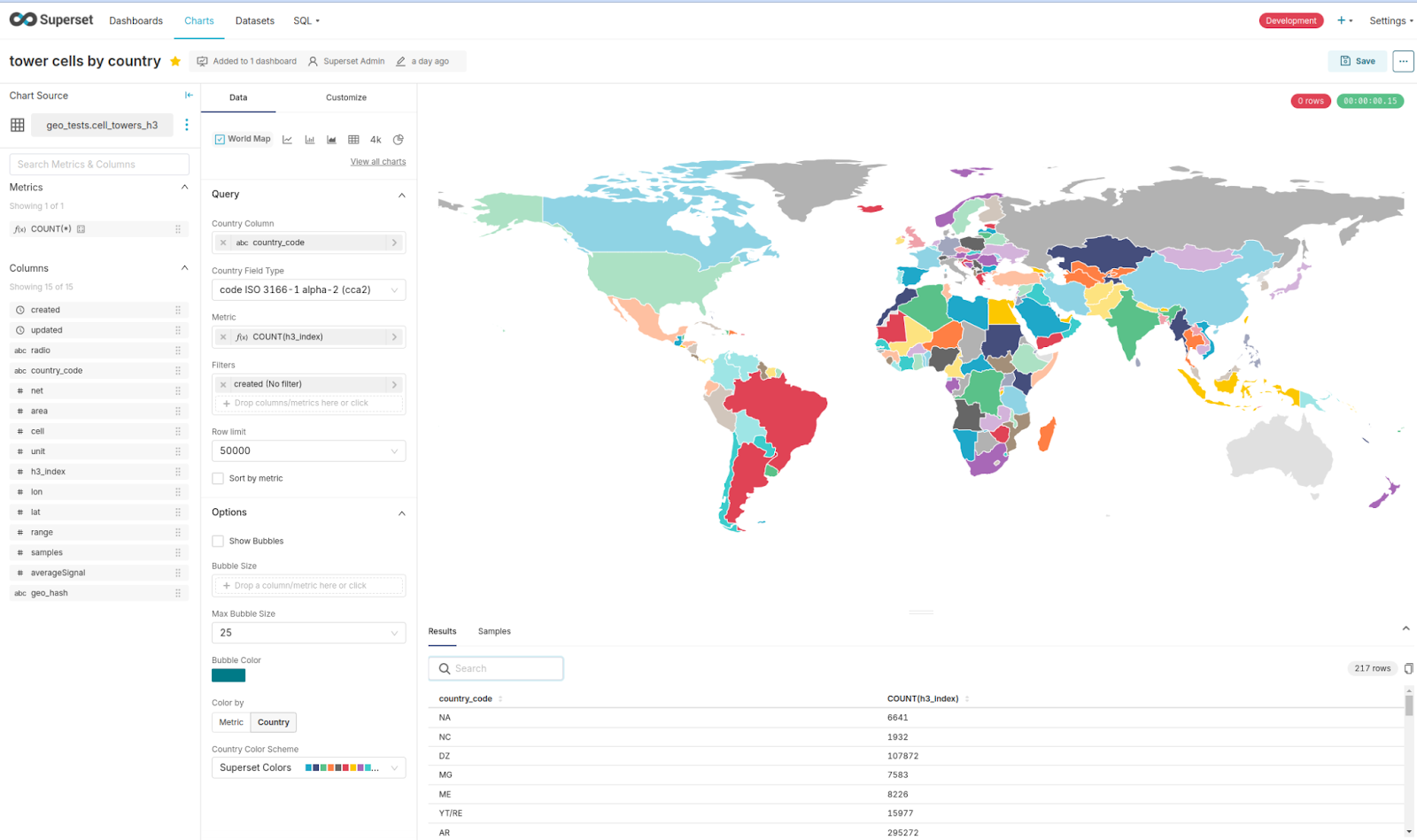
Figures 4 and 5: Number of tower cells per country
For the next visualization we can use the first query from the previous section Finding Nearby Cell Towers with H3, that finds all the cell towers in a radius of 5km from Madrid’s city center. Just create a chart with deck.gl Scatterplot visualization:

After that, specify which columns it will use for latitude and longitude (lat and lon columns) and in the filters tab add a WHERE condition like this one:
h3_index IN (SELECT arrayJoin(h3kRing(geoToH3(-3.707395, 40.415295, 9), 8)))

Figures 5 and 6: Number of cell towers in a radius of 5km from Madrid’s city center.
Another cool visualization is the deck.gl heatmap. We can create a heatmap of the zone coverage in Spain, with zooming capabilities. Let’s add a new chart using the deck.gl heatmap:

After, select the columns for latitude and longitude, as we did for other charts, use count(h3_index) as the weight and add a filter like country_code = ‘ES’:

Figure 7 and 8: Spain mobile network coverage heatmap
Wrap up
The addition of H3 indexing to ClickHouse provides a practical solution for handling large-scale geospatial data more efficiently. By leveraging H3’s hexagonal grid system, ClickHouse simplifies operations that would traditionally rely on more complex latitude and longitude calculations. For those working with substantial geospatial datasets, the combination of ClickHouse and H3 indexing offers an easy and reliable approach to spatial analysis, making it easier to manage and query data effectively. This integration positions ClickHouse as a solid choice for projects requiring both high-speed analytics and geospatial capabilities.
ClickHouse® is a registered trademark of ClickHouse, Inc.; Altinity is not affiliated with or associated with ClickHouse, Inc.