The Mandelbrot Set in… ClickHouse®

During long Christmas evenings you often can finally find time to do something for yourself that you could not afford during the year due to business or family priorities. So did I, which led to an evening playing maths with ClickHouse.

I fell in love with maths and computers when I was at school, and one of my first serious computer programs was a visualization of the Mandelbrot set, written in C++ and i386 assembler. Later on I got “The Fractal Geometry of Nature” book, which is still one of my absolute favourites. 35 years later a lot of things have changed. There are many specialized computer programs for mathematics. But even generic tools like ClickHouse and Grafana can quickly help with the math research that required substantial software development in the past.

The Mandelbrot Set

The Mandelbrot set is one of the most famous mathematical figures in popular culture. It is produced by a very simple algorithm, and yet shows deep mathematical complexity. But it is more known for its beautiful visualizations.

The definition of the Mandelbrot set is very simple.

A complex point c belongs to the Set if
zn+1 =  zn2 + c,  when iterated starting from (0,0) does not run to infinity.

Let’s try to express it in SQL.

First, we will represent complex numbers as tuple datatype tuple(Float64, Float64)

The square of a complex number is calculated as follows (remember, that i is imaginary unit which square equals minus one):

z2= (a + ib)2 = a2 + 2aib - b2= a2 - b2 + i2ab

Therefore, if z and c are tuples, we can calculate z² + c as follows in SQL:

z*z + c = (z.1*z.1 - z.2*z.2 + c.1, 2*z.1*z.2 + c.2)

We also need conditions that would determine the result of an iteration. The simplest approach is the following:

1. If |z_n| > 2, then the point does not belong to the set. Here || represents the modulus of a complex number, i.e. |z|² = a² + b². 
2. If after N iterations |z_n| < 2, we may assume it belongs to the set. Usually 100 iterations are sufficient, and only very close to the border of the Set it may require more iterations for the correct answer.

Geometrically, this condition checks if a point is inside or outside of a circle radius 2 at a complex plane.

There are multiple ways to build iterative processes in ClickHouse SQL. Initially, I tried recursive CTEs as I did in the Collatz conjecture article, but it blew up on a big number of points. So, I used the arrayFold function instead. With arrayFold the algorithm is very simple and easy to read:

with 0.2 as cx,
     0.2 as cy
select arrayFold(z, i -> 
          (z.1*z.1 - z.2*z.2 + cx, 2*z.1*z.2 + cy,
          z.1*z.1 + z.2*z.2<4
          ),
          range(100), (0.0, 0.0, 0)
        )

It runs 100 iterations and returns a final result, and a flag if it belongs to circle radius 2 or not.

Now we may iterate through multiple points on the plane:

with arrayMap(x-> x/10, range(-25, 10)) as xs,
     arrayMap(y-> y/10, range(-10, 10)) as ys            
select arrayJoin(ys) as cy,
       arrayMap (x -> x.3,
       arrayMap(
        cx -> arrayFold(z, i -> 
          (z.1*z.1 - z.2*z.2 + cx, 2*z.1*z.2 + cy,
          z.1*z.1 + z.2*z.2<4
          ),
          range(100), (0.0, 0.0, 0)
        ), 
       xs))
  from system.one

Voilà! We have got an excellent text “picture” with a recognizable shape of the Mandelbrot set:

┌───cy─┬─arrayMap(lambda(tuple(x), tupleElem⋯)), range(100), (0., 0., 0))), xs))─┐
│   -1 │ [0,0,0,0,0,0,0,0,0,0,0,0,0,0,0,0,0,0,0,0,0,0,0,0,0,1,0,0,0,0,0,0,0,0,0] │
│ -0.9 │ [0,0,0,0,0,0,0,0,0,0,0,0,0,0,0,0,0,0,0,0,0,0,0,0,0,0,0,0,0,0,0,0,0,0,0] │
│ -0.8 │ [0,0,0,0,0,0,0,0,0,0,0,0,0,0,0,0,0,0,0,0,0,0,0,1,1,0,0,0,0,0,0,0,0,0,0] │
│ -0.7 │ [0,0,0,0,0,0,0,0,0,0,0,0,0,0,0,0,0,0,0,0,0,0,0,1,1,0,0,0,0,0,0,0,0,0,0] │
│ -0.6 │ [0,0,0,0,0,0,0,0,0,0,0,0,0,0,0,0,0,0,0,0,1,0,1,1,1,1,1,0,0,0,0,0,0,0,0] │
│ -0.5 │ [0,0,0,0,0,0,0,0,0,0,0,0,0,0,0,0,0,0,0,0,1,1,1,1,1,1,1,1,1,0,0,0,0,0,0] │
│ -0.4 │ [0,0,0,0,0,0,0,0,0,0,0,0,0,0,0,0,0,0,0,1,1,1,1,1,1,1,1,1,1,0,0,0,0,0,0] │
│ -0.3 │ [0,0,0,0,0,0,0,0,0,0,0,0,0,0,0,0,0,0,0,1,1,1,1,1,1,1,1,1,1,0,0,0,0,0,0] │
│ -0.2 │ [0,0,0,0,0,0,0,0,0,0,0,0,0,0,1,1,1,0,1,1,1,1,1,1,1,1,1,1,1,0,0,0,0,0,0] │
│ -0.1 │ [0,0,0,0,0,0,0,0,0,0,0,0,0,1,1,1,1,1,1,1,1,1,1,1,1,1,1,1,1,0,0,0,0,0,0] │
│    0 │ [0,0,0,0,0,0,1,1,1,1,1,1,1,1,1,1,1,1,1,1,1,1,1,1,1,1,1,1,0,0,0,0,0,0,0] │
│  0.1 │ [0,0,0,0,0,0,0,0,0,0,0,0,0,1,1,1,1,1,1,1,1,1,1,1,1,1,1,1,1,0,0,0,0,0,0] │
│  0.2 │ [0,0,0,0,0,0,0,0,0,0,0,0,0,0,1,1,1,0,1,1,1,1,1,1,1,1,1,1,1,0,0,0,0,0,0] │
│  0.3 │ [0,0,0,0,0,0,0,0,0,0,0,0,0,0,0,0,0,0,0,1,1,1,1,1,1,1,1,1,1,0,0,0,0,0,0] │
│  0.4 │ [0,0,0,0,0,0,0,0,0,0,0,0,0,0,0,0,0,0,0,1,1,1,1,1,1,1,1,1,1,0,0,0,0,0,0] │
│  0.5 │ [0,0,0,0,0,0,0,0,0,0,0,0,0,0,0,0,0,0,0,0,1,1,1,1,1,1,1,1,1,0,0,0,0,0,0] │
│  0.6 │ [0,0,0,0,0,0,0,0,0,0,0,0,0,0,0,0,0,0,0,0,1,0,1,1,1,1,1,0,0,0,0,0,0,0,0] │
│  0.7 │ [0,0,0,0,0,0,0,0,0,0,0,0,0,0,0,0,0,0,0,0,0,0,0,1,1,0,0,0,0,0,0,0,0,0,0] │
│  0.8 │ [0,0,0,0,0,0,0,0,0,0,0,0,0,0,0,0,0,0,0,0,0,0,0,1,1,0,0,0,0,0,0,0,0,0,0] │
│  0.9 │ [0,0,0,0,0,0,0,0,0,0,0,0,0,0,0,0,0,0,0,0,0,0,0,0,0,0,0,0,0,0,0,0,0,0,0] │
└──────┴─────────────────────────────────────────────────────────────────────────┘

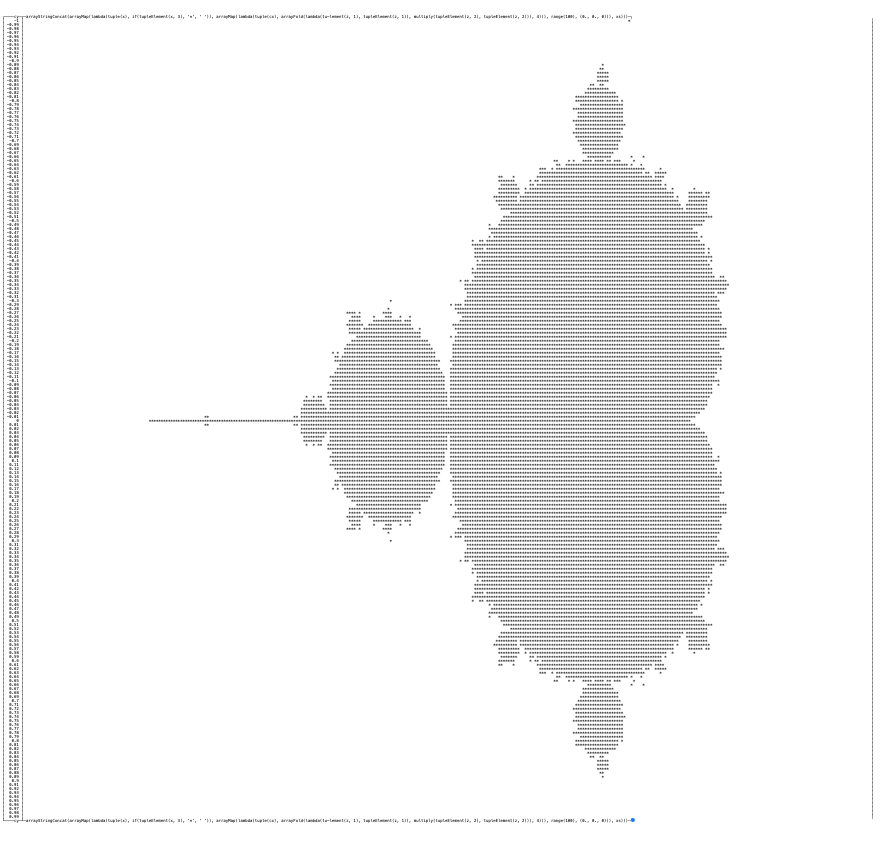
By increasing resolution 10 times and remapping zeros and ones to spaces and asterisks respectively, I could get this fancy one:

Let’s try to add a bit of color using Grafana now.

Visualization with Grafana XY Chart

ClickHouse and Grafana work great together. Altinity is a proud maintainer of the most popular Altinity Grafana data source for ClickHouse with more than 25 million downloads. It can do plot graphs using XY Chart. It requires two columns with XY coordinates, so we will translate the query as follows:

with 0.1 as scale,
     (-2.5, 1.0) as range_x,
     (-1.0, 1.0) as range_y,
     arrayMap(x-> x*scale, range((range_x.1/scale)::Int64, (range_x.2/scale)::Int64)) as xs,
     arrayMap(y-> y*scale, range((range_y.1/scale)::Int64, (range_y.2/scale)::Int64)) as ys
select arrayJoin(ys) as cy,
       arrayJoin(xs) as cx,
       arrayFold(z, i -> 
          (z.1*z.1 - z.2*z.2 + cx, 2*z.1*z.2 + cy,
          if(z.1*z.1 + z.2*z.2>4 and z.3==0, i, z.3),
          ),
          range(1000), (0.0, 0.0, 0::UInt16)
        ).3 as v

Note, that instead of the binary flag, we return an iteration number when a point went out of the bounding circle. We will use it for color.

The query allows easy tuning for range and scale, and produces a dataset with 3 columns:

┌───────────────────cy─┬───────────────────cx─┬──v─┐
│                   -1 │                 -2.5 │  1 │
│                   -1 │  -2.4000000000000004 │  1 │
│                   -1 │  -2.3000000000000003 │  1 │
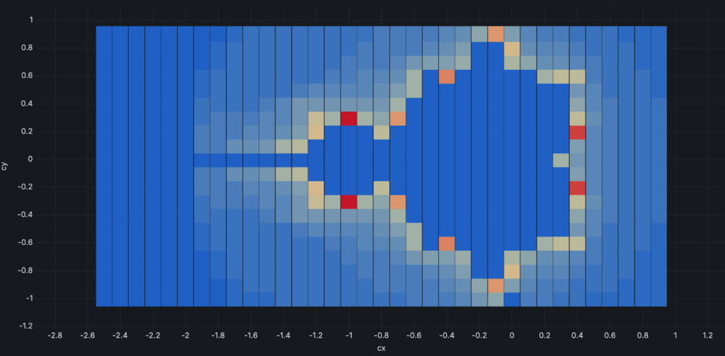
│                   -1 │                 -2.2 │  1 │

We will use the third column as a color. Even the first results were encouraging:

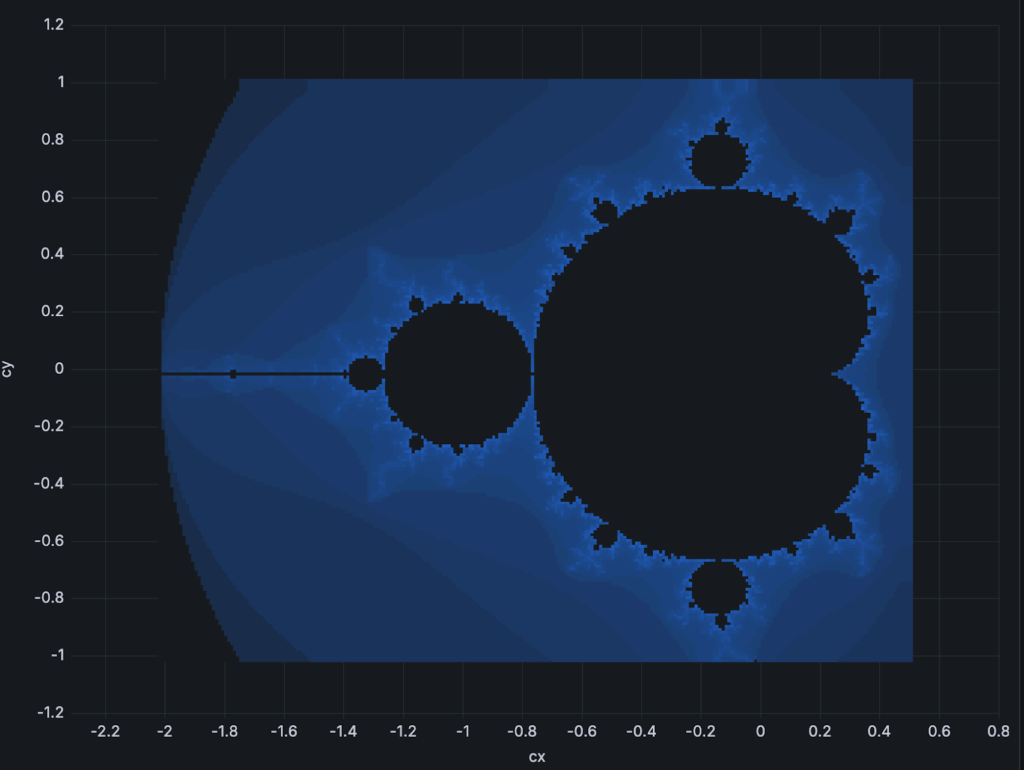
After a bit of tweaking the color palette and color mapping, it started to look almost classic:

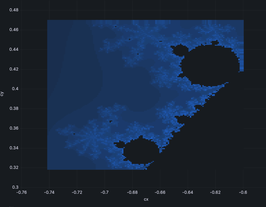
And we can even zoom by adjusting ranges and scale in order to see more examples of self-similarity.

If you want to play around by yourself, the dashboard source code is available at altinity/examples GitHub repository.

Of course, Grafana is not very well suited for interactive exploration of XY space. It also struggles hard when there are many points to display; my browser just freezes. The last two pictures above have resolutions of 200×200 points or slightly more. This is not too much. In the early nineties, I could easily draw higher resolution visualizations with instant refresh time using direct memory access and switching VGA video pages. Needless to say, computers were 1000 times slower back then.

But now it does not require any additional software or programming, since ClickHouse and Grafana are a part of Altinity.Cloud that any user can instantly use.

Final Words

ClickHouse is one of the most versatile and fun-to-use databases in the world. After 9 years, it still amazes me with its power and speed. It can do everything from real-time ingest, scanning terabytes of data, or playing with math puzzles. In this article, I showed how it can be used in order to generate and visualize the famous Mandelbrot set. Please join the joy and share your fun visualizations using ClickHouse!