Navigating Object Storage and Iceberg Data Lakes with ClickHouse® SQL

Uniform access to data through SQL is a superpower of modern databases. This capability extends from tables to system catalogs to data on file systems. The latest frontier is data lakes, which contain an increasing volume of data in Apache Parquet files organized under open table formats like Apache Iceberg and Delta Lake in object storage. ClickHouse offers especially powerful capabilities in this area.
We’ll prove the point by using ClickHouse SQL to examine every aspect of an Iceberg table, from enumeration of files to queries on Iceberg REST catalogs. The Iceberg table format is a perfect example to show off ClickHouse capabilities. Iceberg tables have complex metadata and multiple file types. With simple SQL queries, the information becomes easily visible.
This capability is useful for many reasons, of which two are especially important. First, many applications write and read data in Iceberg tables. It’s important to be able to examine tables directly when debugging problems, optimizing performance, or just trying to understand what’s there. Second, ClickHouse SQL is a great foundation for tools that manage Iceberg tables. There’s no reason to bring in extra tools outside the database. You can build on ClickHouse.
How Are Iceberg Tables Structured?
Let’s start with a quick primer on Apache Iceberg table structure. This will help readers understand how things are put together. Iceberg files are generally loaded using a path that includes the table name and divides into separate paths for data and metadata. It looks like the following.

These are conventions, and not every Iceberg table follows them. It depends on the tool used to write the table as well as user choices. For example, it’s possible to put data files under a different path from metadata files. You can also add additional files. Dremio and some other implementations add a file named version-hint.text to locate the latest table version. Finally there’s no hard and fast rule for naming files. Instead, we locate files by reading the Iceberg table metadata, not by their names.
The files we are touring in this article were exported from ClickHouse using the new Project Antalya ALTER TABLE EXPORT COMMAND. I imported them into Iceberg using the Altinity Ice utility invoked as follows. The command specifies the partitioning and sort order. We will see this information in the Iceberg metadata data.
ice insert default.ontime -p --thread-count=12 \
 --no-copy \
 --partition='[{"column":"Year"}]' \
 --sort='[{"column":"Carrier", "desc":false}, {"column":"FlightDate", "desc":false}]' \
 --assume-sorted \
"s3://my-bucket/default/ontime/data/*/*.parquet"
Finding Out What’s in Object Storage
Let’s start with the basics: files on S3 object storage. Speaking of which, what files are in our Iceberg table? We can start with a simple query to enumerate the full path of each file.
SELECT _path
FROM s3('s3://my-bucket/default/ontime/**', One)
ORDER BY _path ASC FORMAT Vertical

Row 1:
──────
_path: my-bucket/default/ontime/data/Year=1987/1987_1_1_0_EBFB...C1C4.1.parquet
Row 2:
──────
_path: my-bucket/default/ontime/data/Year=1987/1987_3_3_0_E995...6C1.1.parquet
Row 3:
──────
_path: my_bucket/default/ontime/data/Year=1987/commit_1987_1_1_0_EBF...C1C4
Our query uses the s3() table function and leans on three key features to extract relevant information.
- Virtual columns. The _path column gives the full path to the file in object storage.
- Wildcards. The ‘**” wildcard matches any file that starts with the prefix.
- The One input format. This is a special format that reads file metadata only, not the rows inside it. The result is one output row for each file.
We can add more virtual columns to get additional metadata. Here is a query showing all of those supported for files in S3.
SELECT _path, _file, _size, _time, _etag
FROM s3('s3://my-bucket/default/ontime/data/Year=1987/1987_1_1_0_EBFB...C1C4.1.parquet', One)
FORMAT Vertical

Row 1:
──────
_path: my-bucket/default/ontime/data/Year=1987/1987_1_1_0_EBFB...C1C4.1.parquet
_file: 1987_1_1_0_EBFB...C1C4.1.parquet
_size: 12257633 -- 12.26 million
_time: 2026-02-21 12:50:44
_etag: "58c79fbcd1dd8a0b850ae10293bdc905"
Here’s a quick summary of each virtual column derived from reading ClickHouse source code. (The docs were ambiguous. Thanks for helping, Claude!)
| Virtual Column | Description |
| _path | Full path to file |
| _file | Filename only (without directory path) |
| _size | File size in bytes |
| _time | Last modified time |
| _etag | ETag (entity tag) of the file, which is a hash of the stored object |
We can also gather file data in a more succinct form using aggregation. How many file types are in the table and how many files does each one have? Here is the query to find out.
SELECT extract(_file, '.*\\.(.*)$') AS file_type, count()
FROM s3('s3://my-bucket/default/ontime/**', One)
GROUP BY file_type
ORDER BY file_type ASC

   ┌─file_type─┬─count()─┐
1. │           │      13 │
2. │ avro      │       2 │
3. │ json      │       2 │
4. │ parquet   │      13 │
   └───────────┴─────────┘
This is interesting. What are the files without data types? It turns out they are generated during export of parts from ClickHouse to S3 object storage. They aren’t part of the Iceberg format, and the Altinity Ice Catalog will eventually clean them up automatically as part of table maintenance. Let’s see what’s in one of them.
SELECT * FROM s3('s3://my-bucket/default/ontime/data/Year=1987/commit_1987_3_3_0_E995...F6C1')

Row 1:
──────
default/ontime/data/Year: 1987/1987_3_3_0_E995...F6C1.1.parquet
Year:                     1987
We see the data, but what kind of file are we looking at? ClickHouse does not give up this secret easily. However, if you add SETTINGS send_logs_level = ‘debug’ to the query and search the resulting log messages, you’ll find that it is the TSKV input format. The clickhouse-client output is shown below.
SELECT * FROM s3('s3://my-bucket/default/ontime/data/Year=1987/commit_1987_3_3_0_E995...F6C1')
SETTINGS send_logs_level = 'debug'
. . .
[chi-my-swarm-my-swarm-0-0-0] 2026.02.24 16:10:08.342674 [ 806 ]  {dab4f667-b89d-49d2-9f56-e10810779f95} <Debug> executeQuery: (from [::ffff:10.129.152.255]:34032, user: swarm_access, initial_query_id: 138bb6df-afbe-4e87-82c6-3a9fa8172122) (query 1, line 1) SELECT __table1.`default/ontime/data/Year` AS `default/ontime/data/Year`, __table1.Year AS Year FROM s3Cluster('my-swarm', 's3://my-bucket/default/ontime/data/Year=1987/commit_1987_3_3_0_E9959EB7178905EA836AFB9D8645F6C1', 'TSKV', '`default/ontime/data/Year` Nullable(String), `Year` Int64') AS __table1 SETTINGS send_logs_level = 'debug' (stage: WithMergeableState)
(I said ClickHouse does not give up the secret easily!)
The fact you can read file data without even knowing the format is incredibly handy. ClickHouse’s ability to handle different file formats automatically is quite amazing.
Let’s move up a level and ask one more question. We have the path to one Iceberg table already. Are there others in the bucket? We can find out with a bit of regular expression hackery. There are five tables.
SELECT DISTINCT arrayStringConcat(table_array, '.') AS table_name
FROM
(
    SELECT
        extract(_path, '[a-zA-Z0-9]*/(.*)/metadata/.*$') AS table_path,
        splitByChar('/', table_path) AS table_array
    FROM s3('s3://my-bucket/**', One)
    WHERE length(table_path) > 0
)
ORDER BY table_name ASC

   ┌─table_name───────────────────────────┐
1. │ aws-public-blockchain.btc            │
2. │ aws-public-blockchain.btc_live       │
3. │ aws-public-blockchain.btc_ps_by_date │
4. │ default.ontime                       │
5. │ ssb.lineorder_wide                   │
   └──────────────────────────────────────┘
One final note! If you are using a Project Antalya build, you should know about the use_object_storage_list_objects_cache setting. It caches calls to enumerate lists of files on S3-compatible storage. This speeds up queries on buckets with many files substantially but means you may not see recently added files. If you think this is happening you can turn it off as shown in the following example.
SELECT DISTINCT _path, _file, _size, _time, _etag
FROM s3('s3://my-bucket/default/ontime/**', One)
SETTINGS use_object_storage_list_objects_cache = 0
Looking at Parquet File Data and Metadata
Our Iceberg table stores data in Parquet files, the most popular columnar file format for data lakes. Parquet format is fully documented here, in case you want to do some background reading. Meanwhile, ClickHouse can help us learn about what’s inside individual Parquet files very quickly. For example, we can count the rows as follows. In fact this file is just like a SQL table. You can run any query on it you like.
SELECT count() FROM s3('s3://my-bucket/default/ontime/data/Year=1993/1993_37_37_0_8532...9889.1.parquet')

   ┌─count()─┐
1. │  740075 │
   └─────────┘
Just like a SQL table we can also describe the Parquet file columns.
DESCRIBE TABLE s3('s3://my-bucket/default/ontime/data/Year=1993/1993_37_37_0_8532...9889.1.parquet')
FORMAT Vertical

Row 1:
──────
name:               Year
type:               Nullable(UInt16)
...
It’s convenient that ClickHouse fetches the type information but we can also get it directly from the Parquet file. The format is fully self-describing and the following query dumps everything.
SELECT *FROM s3('s3://my-bucket/default/ontime/data/Year=1993/1993_37_37_0_8532...9889.1.parquet', ParquetMetadata)The ParquetMetadata input format is a key piece of magic that makes the queries work. It dumps the metadata from Parquet instead of the data. Unfortunately, the result is an ugly mess with nested definitions of columns and row groups. Fortunately, it only takes a small effort to make the output more civilized.
First, let’s let ClickHouse describe the complete format of the metadata. It will even show nested data structures.
DESCRIBE TABLE s3('s3://my-bucket/default/ontime/data/Year=1993/1993_37_37_0_8532...9889.1.parquet', ParquetMetadata)

Row 1:
──────
name:               num_columns
type:               UInt64
. . .
Once we have names for columns and the nested structures within them, it’s possible to create queries that make things human readable. Let’s start with general information about the Parquet file contents.
SELECT
    _file, num_columns, num_rows, num_row_groups,
    format_version, total_uncompressed_size, total_compressed_size
FROM s3('s3://my-bucket/default/ontime/data/Year=1993/1993_37_37_0_8532...9889.1.parquet', ParquetMetadata)
FORMAT Vertical

Row 1:
──────
_file:                   1993_37_37_0_8532...9889.1.parquet
num_columns:             109
num_rows:                740075
num_row_groups:          1
format_version:          2
total_uncompressed_size: 25352826 -- 25.35 million
total_compressed_size:   10847364 -- 10.85 million
Next, let’s look at the column definitions. Thanks to the handy ARRAY JOIN operation we can unroll the nested column definitions.
SELECT
    col.name AS name,
    col.physical_type AS physical_type,
    col.logical_type AS logical_type,
    col.compression AS compression,
    col.total_uncompressed_size AS total_uncompressed_size,
    col.total_compressed_size AS total_compressed_size,
    col.space_saved AS space_saved,
    col.encodings AS encodings
FROM s3('s3://my-bucket/default/ontime/data/Year=1993/1993_37_37_0_8532...9889.1.parquet', ParquetMetadata)
ARRAY JOIN columns AS col
FORMAT Vertical

Row 1:
──────
name:                    Year
physical_type:           INT32
logical_type:            Int(bitWidth=16, isSigned=false)
compression:             ZSTD
total_uncompressed_size: 69
total_compressed_size:   101
space_saved:             -46.38%
encodings:               ['PLAIN','RLE_DICTIONARY']
. . .
If you like to nerd out on data types, this is gold. It’s beautiful to see that Parquet supports unsigned integer types. It also defaults (in this case) to ZSTD compression.
Parquet stores data in row groups, which are sets of rows in columnar format. They are like granules in ClickHouse MergeTree tables. We can get exact information about each row group.
SELECT
    rg.file_offset AS file_offset,
    rg.num_columns AS num_columns,
    rg.num_rows AS num_rows,
    rg.total_uncompressed_size AS total_uncompressed_size,
    rg.total_compressed_size AS total_compressed_size
FROM s3('s3://my-bucket/default/ontime/data/Year=1993/1993_37_37_0_8532...9889.1.parquet', ParquetMetadata)
ARRAY JOIN row_groups AS rg
FORMAT Vertical

Row 1:
──────
file_offset:             4
num_columns:             109
num_rows:                740075
total_uncompressed_size: 25352826 -- 25.35 million
total_compressed_size:   10847364
Our file is small so there is just one row group. We can even reach into the row group and get information about each column in the group, such as the min and max values of the column. Here’s how to do it.
SELECT
    file_offset AS offset, col.name AS name,
    col.statistics.min AS min, col.statistics.max AS max
FROM
(
    SELECT
        rg.file_offset AS file_offset,
        rg.columns AS columns
    FROM s3('s3://my-bucket/default/ontime/data/Year=1993/1993_37_37_0_8532...9889.1.parquet', ParquetMetadata)
    ARRAY JOIN row_groups AS rg
)
ARRAY JOIN columns AS col

     ┌─offset─┬─name─────────────────┬─min──────────────┬─max──────────────┐
  1. │      4 │ Year                 │ 1993             │ 1993             │
  2. │      4 │ Quarter              │ 1                │ 4                │
  3. │      4 │ Month                │ 1                │ 12               │
  4. │      4 │ DayofMonth           │ 1                │ 31               │
  5. │      4 │ DayOfWeek            │ 1                │ 7                │
  6. │      4 │ FlightDate           │ 8401             │ 8765             │
. . .
At this point we’ve learned a great deal about the Parquet file contents, and further inquiry might exceed the bounds of good taste. The metadata is now at your disposal. We’ll meanwhile turn to look at Iceberg table metadata.
Finding Out What’s in an Iceberg Table
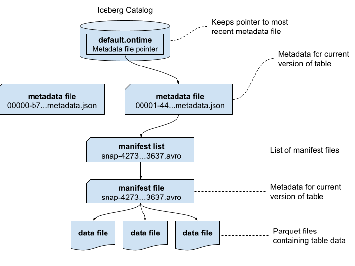
Iceberg metadata is stored in a combination of JSON and Avro files. Let’s trace through and see what’s inside. To make the results easier to understand, we’ll first start by showing how the metadata files are related. This is a simpler version of the picture provided by the Iceberg specification that uses real file names.
It’s a good time to point out that the Apache Iceberg project provides a full table specification that covers the contents of each of the above files, including precise definitions of each field. Many fields are self-explanatory, but if in doubt you now have a source for full answers.
Let’s first start by enumerating the metadata files. We will also sort them by descending time.
SELECT
    _path,
    _time
FROM s3('s3://my-bucket/default/ontime/metadata/**', One)
ORDER BY _time DESC
FORMAT Vertical

Row 1:
──────
_path: my-bucket/default/ontime/metadata/00001-4457...6779.metadata.json
_time: 2026-02-21 14:08:47

Row 2:
──────
_path: my-bucket/default/ontime/metadata/snap-4273...3637.avro
_time: 2026-02-21 14:08:46
. . .
Next, we want to find the schema of the metadata.json files using the last file written. (If you pick the first file there is a chance it may not contain all schema, because it may not have any manifests yet.)
DESCRIBE s3('s3://my-bucket/default/ontime/metadata/00001-4457...6779.metadata.json')
FORMAT Vertical
Let’s run a query to check the main properties of the table. We won’t bother to unroll the nested structures like partition specs and sort orders. Instead, we can print them in prettified JSON, which is quite readable.
SELECT
    `format-version`,
    location,
    `last-sequence-number`,
    `last-updated-ms`,
    `partition-specs`,
    `sort-orders`
FROM s3('s3://my-bucket/default/ontime/metadata/00001-4457...6779.metadata.json')
FORMAT PrettyJSONEachRow

{
    "format-version": 2,
    "location": "s3:\/\/my-bucket\/default\/ontime",
    "last-sequence-number": 1,
    "last-updated-ms": 1771682926743,
    "partition-specs": [
        {
            "fields": [
                {
                    "field-id": 1000,
                    "name": "Year",
                    "source-id": 1,
                    "transform": "identity"
                }
                ...
It’s more interesting to unroll the column definitions into a proper table. Here’s a query to do that.
SELECT
    field.id AS id,
    field.name AS name,
    field.required AS required,
    field.type AS type
FROM s3('s3://my-bucket/default/ontime/metadata/00001-4457...6779.metadata.json')
ARRAY JOIN tupleElement(schemas[1], 'fields') AS field
ORDER BY id ASC

     ┌──id─┬─name─────────────────┬─required─┬─type─────┐
  1. │   1 │ Year                 │ true     │ int      │
  2. │   2 │ Quarter              │ true     │ int      │
  3. │   3 │ Month                │ true     │ int      │
  4. │   4 │ DayofMonth           │ true     │ int      │
  5. │   5 │ DayOfWeek            │ true     │ int      │
  6. │   6 │ FlightDate           │ true     │ date     │
  . . .
This query works if you don’t change the schema, in which case there is just one set of columns However, if the schema *does* change there will be multiple schemas and you might not get the right one. We’ll leave that as a challenge for energetic readers.
We can move away from the Iceberg schema to find out which files belong to the table. The first thing to do is find the manifest lists, which is exactly what this query does.
SELECT
    snap.`manifest-list` AS manifest_list,
    snap.`schema-id` AS schema_id,
    snap.`sequence-number` AS sequence_number,
    snap.`snapshot-id` AS snapshot_id
FROM s3('s3://my-bucket/default/ontime/metadata/00001-4457...6779.metadata.json')
ARRAY JOIN snapshots AS snap
FORMAT Vertical

Row 1:
──────
manifest_list:   s3://my-bucket/default/ontime/metadata/snap-4273...3637.avro
schema_id:       0
sequence_number: 1
snapshot_id:     4273857594351972880
The full path for the single manifest list is shown in the output. It’s encoded in Avro, which is a self-describing columnar format like Parquet. We can read the file contents as follows.
SELECT * FROM s3('s3://my-bucket/default/ontime/metadata/snap-42738...3637.avro')
FORMAT Vertical

Query id: d8c7f7be-910d-46f1-8c5f-236b244783dc

Row 1:
──────
manifest_path:        s3://my-bucket/default/ontime/metadata/e0ea...3637-m0.avro
manifest_length:      22087
partition_spec_id:    0
. . .
There is just one manifest file but it has a lot of nested information. We’ll read that using a query that breaks out the nested information in a more human-readable format.
SELECT status, snapshot_id, sequence_number, file_sequence_number,
  data_file.content AS content,
  data_file.file_path AS file_path,
  data_file.file_format AS file_format,
  data_file.partition AS partition
FROM
s3('s3://my-bucket/default/ontime/metadata/e0ea...3637-m0.avro')
FORMAT Vertical

Row 1:
──────
status:               1
snapshot_id:          4273857594351972880
sequence_number:      ᴺᵁᴸᴸ
file_sequence_number: ᴺᵁᴸᴸ
content:              0
file_path:            s3://my-bucket/default/ontime/data/Year=1987/1987_1_1_0_EBFB...C1C4.1.parquet
file_format:          PARQUET
partition:            (1987)
. . .
The manifest list is an interesting and critically important file. It provides statistics that ClickHouse uses to prune partitions and skip files within partitions. We can see already that our Parquet files are assigned to the expected partitions, which is comforting. Ensuring statistics are correct is a high priority so that queries run fast and return the right results.
Finally, we showed previously how to locate Iceberg tables using regex expressions on file names. We can also find the paths by scanning metadata.json files, as shown in the following example.
SELECT DISTINCT location
FROM s3('s3://my-bucket/**/*.metadata.json')
ORDER BY location
SETTINGS input_format_json_use_string_type_for_ambiguous_paths_in_named_tuples_inference_from_objects = 1
   ┌─location────────────────────────────────────────────┐
1. │ s3://my-bucket/aws-public-blockchain/btc_live       │
2. │ s3://my-bucket/default/ontime                       │
3. │ s3://my-bucket/aws-public-blockchain/btc            │
4. │ s3://my-bucket/aws-public-blockchain/btc_ps_by_date │
5. │ s3://my-bucket/ssb/lineorder_wide                   │
   └─────────────────────────────────────────────────────┘
Note the input_format_json_use_string_type_for_ambiguous_paths… setting on this query. Depending on their content metadata.json files may have different schemas. This setting tells ClickHouse to reconcile ambiguous paths in JSON. Without it your query may fail.
Working With Iceberg REST Catalogs
Not everything in Iceberg tables is a file in object storage. Iceberg REST catalogs track the current location of file metadata, which saves you from having to scan Iceberg metadata.json files to find the most current table snapshot.
We can query Iceberg REST catalogs using the ClickHouse url() functions. You’ll need to have a bearer token or another means of authentication to the catalog. Here’s an example of querying the available namespaces for Iceberg tables.
SELECT namespace
FROM url('http://ice-rest-catalog:5000/v1/namespaces', headers('Authorization' = 'Bearer someTokenString'))
ARRAY JOIN namespaces AS namespace

   ┌─namespace─────────────────┐
1. │ ['aws-public-blockchain'] │
2. │ ['default']               │
3. │ ['ssb']                   │
   └───────────────────────────┘
We can now query the tables within the default namespace.
SELECT
    `table`.name AS table_name,
    `table`.namespace AS table_namespace
FROM url('http://ice-rest-catalog:5000/v1/namespaces/default/tables', headers('Authorization' = 'Bearer someTokenString'))
ARRAY JOIN identifiers AS `table`

   ┌─table_name─┬─table_namespace─┐
1. │ ontime     │ ['default']     │
   └────────────┴─────────────────┘
Finally, we can look up the location of the current metadata.json file for the ontime table.
SELECT `metadata-location`
FROM url('http://ice-rest-catalog:5000/v1/namespaces/default/tables/ontime', headers('Authorization' = 'Bearer someTokenString'))
FORMAT Vertical

Row 1:
──────
metadata-location: s3://my-bucket/default/ontime/metadata/00001-4457...6779.metadata.json
There is much more information available from this last call. The REST response contains data from the metadata.json, so you don’t have to read the file directly. To see names of the available fields you can use the following handy DESCRIBE invocation.
DESCRIBE TABLE
(
    SELECT *
    FROM url('http://ice-rest-catalog:5000/v1/namespaces/default/tables/ontime', headers('Authorization' = 'Bearer someTokenString'))
)
For more information on Iceberg REST API calls, check out the official specification online.
Conclusion
ClickHouse SQL offers a comprehensive and flexible solution to reading both data as well as metadata from data lakes, including Iceberg tables. We’ve shown how ClickHouse can help you quickly understand the structure and data in Iceberg tables. Its ability to read complex structures across JSON, Avro, and Parquet using simple SQL queries is nothing short of amazing.
ClickHouse SQL is also a great basis for Iceberg table management tools, which can now operate without needing direct access to files, object storage, or Iceberg REST catalogs. We will illustrate some of the things you can build on this foundation in future blog articles.
If you have further questions about this article or any aspect of using ClickHouse with Iceberg data lakes, please contact us or join our Slack workspace to ask questions. We look forward to hearing from you.
ClickHouse® is a registered trademark of ClickHouse, Inc.; Altinity is not affiliated with or associated with ClickHouse, Inc.