Connecting ClickHouse® to Apache Kafka®


Apache Kafka® is an open-source distributed event-streaming platform used by millions around the world. ClickHouse has a Kafka table engine that ties Kafka and ClickHouse together. In this post we’ll cover how to connect a ClickHouse® cluster to a Kafka server. With the connection set up, we’ll create a complete application that shows how ClickHouse and Kafka work together.
The steps we’ll go through are:
- Look at the architecture of our sample application
- Use
ngrokanddocker composeto create a Kafka server onlocalhostand make it visible to the internet - Use the Altinity Cloud Manager® (ACM) to define a Kafka server connection and test it
- Use the ACM to create the ClickHouse infrastructure (tables and materialized views) that uses the connection to the Kafka server
- Run a simple command-line application that generates JSON documents and puts them on the Kafka topic
- Use the ACM to run ClickHouse analytics queries against the live data streaming in from Kafka.
So that’s the plan. Let’s get started!
If you love ClickHouse®, Altinity can simplify your experience with our fully managed service in your cloud (BYOC) or our cloud and 24/7 expert support. Learn more.
Our demo architecture
The architecture looks like this:
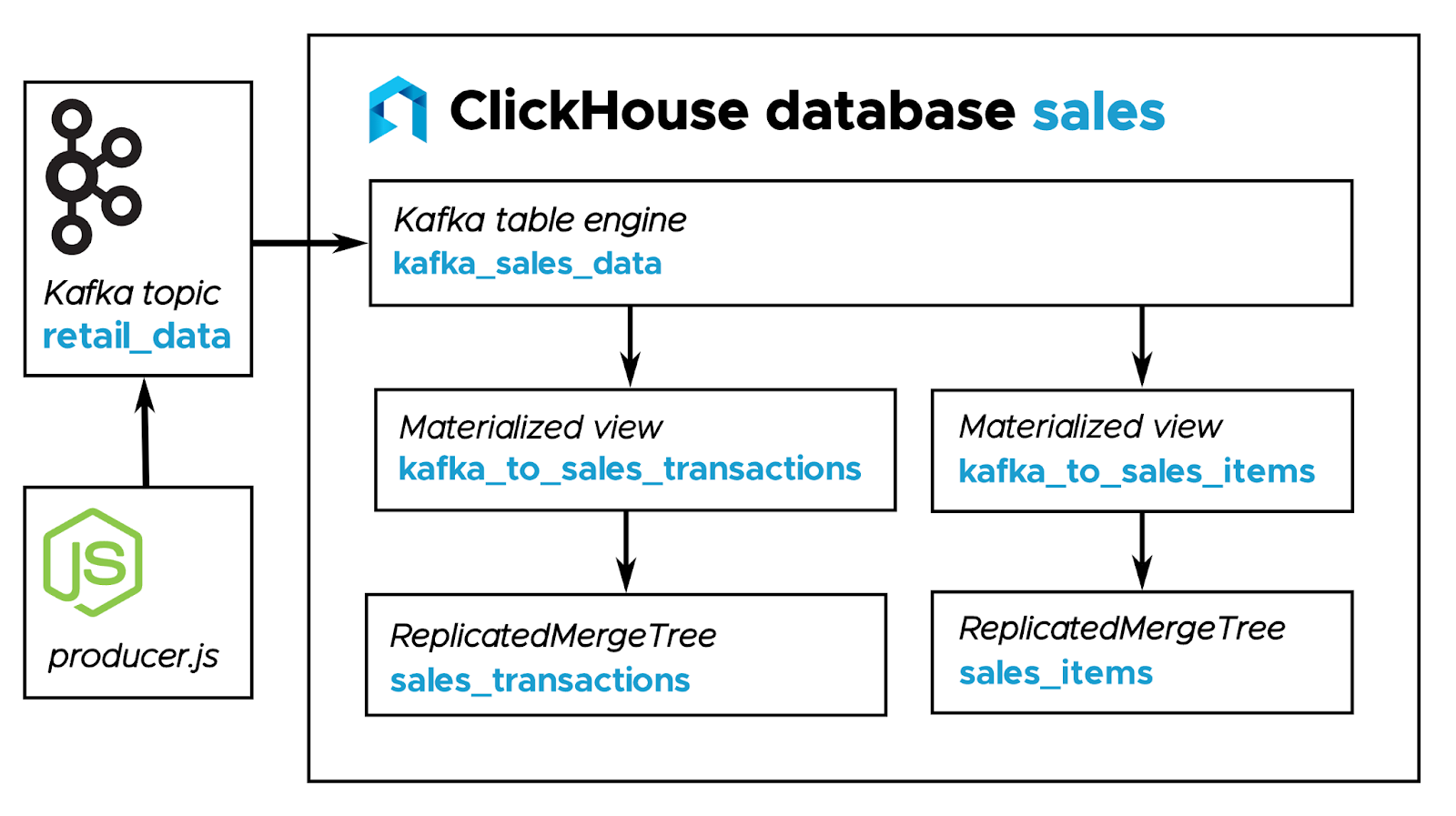
Figure 1. Using Kafka and ClickHouse together
We have a Kafka server that hosts the retail_data topic. We also have a simple Node.js application, producer.js, that generates JSON documents and puts them on the retail_data topic. From there, everything happens in the sales database in our ClickHouse cluster. We have kafka_sales_data, a table that uses the Kafka engine to collect all the data that goes to the topic. From there, we have two ReplicatedMergeTree tables (sales_transactions and sales_items) that are populated by two materialized views (kafka_to_sales_transactions and kafka_to_sales_items).
As for the data, producer.js generates JSON documents that look like this:
{
  "transaction_id": "T43379",
  "customer_id": "C004",
  "timestamp": "2024-09-12T16:16:38.935Z",
  "items": [
    {
      "item_id": "I005",
      "quantity": 3,
      "price": 100
    },
    {
      "item_id": "I001",
      "quantity": 1,
      "price": 40
    }
  ],
  "total_amount": 340,
  "store_id": "S001"
}
Listing 1. An example of the JSON documents we’ll be working with
Each randomly generated document represents a sale of some number of items to a particular customer at a particular store. In this example, customer C004 went to store S001 and bought three of item I005 at $100 each and one of item I001 at $40, for a total of $340. We’ll look at the structure of the tables later.
Setting up ngrok
As mentioned above, we’re running everything on localhost here. We’ll use a free ngrok account to set up a secure tunnel from the outside world into the port of our Kafka server. That means our ClickHouse cluster running in Altinity.Cloud will be able to access our Kafka server running on localhost. (There are lots of other ways to host Kafka, of course; feel free to deploy it however you like.)
The ngrok command makes it simple:
ngrok tcp 9092
You’ll see a display something like this:
ngrok

Route traffic by anything: https://ngrok.com/r/iep
Session Status                online
Account                       Doug Tidwell (Plan: Pro)
Version                       3.18.4
Region                        United States (us)
Latency                       47ms
Web Interface                 http://127.0.0.1:4040
Forwarding                    tcp://X.tcp.ngrok.io:XXXXX -> localhost:9092
At this point, ngrok is listening for TCP traffic on port XXXXX at X.tcp.ngrok.io. We’ll set up a Kafka server that listens on port 9092 on localhost; whenever ClickHouse sends a request from Altinity.Cloud to the ngrok.io address, it’ll be rerouted to our local Kafka server. (BTW, yr author has a Pro account, but this works with a free account. I promise.)
Starting a Kafka server
Starting a Kafka server is as easy as running docker compose. Here’s the docker-compose.yml file we’ll use::
services:
  zookeeper:
    image: bitnami/zookeeper:latest
    container_name: zookeeper
    environment:
      - ALLOW_ANONYMOUS_LOGIN=yes
    ports:
      - "2181:2181"
  kafka:
    image: bitnami/kafka:latest
    container_name: kafka
    depends_on:
      - zookeeper
    environment:
      - KAFKA_CFG_ZOOKEEPER_CONNECT=zookeeper:2181
      - KAFKA_CFG_LISTENERS=PLAINTEXT://0.0.0.0:9092
      - KAFKA_CFG_ADVERTISED_LISTENERS=PLAINTEXT://X.tcp.ngrok.io:XXXXX
      - ALLOW_PLAINTEXT_LISTENER=yes
    ports:
      - "9092:9092"
    volumes:
      - kafka_data:/bitnami/kafka
volumes:
  Kafka_data:
Listing 2. The docker-compose.yml file that starts the Kafka server
The docker-compose.yml file is available in the Altinity Examples repo.
Before starting the containers, replace the value of KAFKA_CFG_ADVERTISED_LISTENERS with the ngrok URL. Once that’s done, just run docker compose up -d:
docker compose up -d
[+] Running 4/4
 ✔ kafka Pulled                                                      20.6s
   ✔ d7b8f2f517c1 Pull complete                                      19.3s
 ✔ zookeeper Pulled                                                  17.0s
   ✔ 886d5ad2fa31 Pull complete                                      15.8s
[+] Running 4/4
 ✔ Network docker-with-zookeeper_default      Created                 0.0s
 ✔ Volume "docker-with-zookeeper_kafka_data"  Created                 0.0s
 ✔ Container zookeeper                        Started                 0.7s
 ✔ Container kafka                            Started                 0.2s
So our Kafka server is up and running! Now let’s create a topic.
Creating a topic on our Kafka server
The Kafka server comes with a number of useful command-line utilities; we’ll use kafka-topics.sh to create our topic. And docker compose makes it easy. First, we’ll create the topic:
docker compose exec kafka kafka-topics.sh --create --topic retail_data --bootstrap-server localhost:9092
Created topic retail_data.
This executes the command kafka-topics.sh --create on the container named kafka. Here we’re using it to create the topic retail_data on localhost. (Ignore any warning messages about topic names that contain periods or underscores.) Let’s run kafka-topics.sh --list to make sure our topic was created correctly:
docker compose exec kafka kafka-topics.sh --list --bootstrap-server localhost:9092
retail_data
(As an aside, since we’re running everything locally, using localhost:9092 as the server address works fine. But using the ngrok URL via --bootstrap-server X.tcp.ngrok.io:XXXXX works too.)
So. Everything looks good on the Kafka side; now we’ll move on to ClickHouse.
Connecting ClickHouse to Kafka servers
ClickHouse’s Kafka table engine extracts data from a Kafka topic. The vast majority of the details of the connection are abstracted away with the engine. To do that, we’ll use the ACM to create a named collection in a ClickHouse XML configuration file. Each collection contains the parameters needed to connect to a particular Kafka server and a particular topic on that server. The collections are stored inside XML files in the config.d directory (/etc/clickhouse-server/config.d).
Here’s a simple named collection:
<clickhouse>
  <named_collections>
    <localhost>
      <kafka_broker_list>X.tcp.ngrok.io:XXXXX</kafka_broker_list>
      <kafka_topic_list>retail_data</kafka_topic_list>
      <kafka_group_name>retail_data</kafka_group_name>
    </localhost>
  </named_collections>
</clickhouse>
This defines a named collection called localhost. We can use the collection name when we create a Kafka table engine inside ClickHouse. (BTW, the ClickHouse CREATE NAMED COLLECTION command can create a collection as well, but the ACM’s approach is much simpler.)
So let’s look at how the Altinity Cloud Manager makes it easy to create the named collection above. In the ACM, open the cluster view for your ClickHouse cluster and click Kafka Connections on the CONFIGURE menu:

Figure 2. The Configure Kafka Connections menu item
The settings in Figure 3 create an XML file named kafka.xml and a named collection named localhost:

Figure 3. Configuring a connection to a Kafka server
If we click the CHECK button, the ACM will attempt to connect to the Kafka server with the details defined here. If everything works, you’ll see a dialog like this:

Figure 4. Results of a successful connection to a Kafka server
The kafka_broker_list element defines the URL(s) for the Kafka server. We only have one here, but this can be a comma-separated list of multiple endpoints. The kafka_topic_list is a comma-separated list of the Kafka topic(s) we want ClickHouse to monitor. In this simple case, the kafka_group_name is the same. See the official Kafka documentation for more details on working with topics and groups; that goes way beyond our scope here.
Click the SAVE INTO SETTINGS button to add the localhost named collection to the settings file.
The Kafka server we’ve set up here has absolutely no authentication whatsoever. Obviously most Kafka servers aren’t deployed so irresponsibly; fortunately the ACM makes it easy to define advanced parameters. For example, a connection to a Confluent Kafka server might look like this:

Figure 5. A connection to a Kafka server with authentication parameters
The ADD OPTION and ADD PRESET buttons let you add more parameters as needed. See the Altinity Cloud Manager Kafka Connections documentation for all the details of the ACM user interface. For even more detailed information, see the article Adjusting librdkafka settings in the Altinity Knowledge Base for everything you’ll ever need to know about connecting ClickHouse and Kafka.
The ACM lets you define multiple connections in a single file. If the Confluent parameters above worked, you can save both connections in config.d/kafka.xml:

Figure 6. A Kafka settings file with two connections
Setting up ClickHouse
Now that we’ve got our Kafka server set up, we need to create the ClickHouse resources in Figure 1 above. They are:
- A table with a
Kafkaengine. That table will use the Kafka configuration we set up to look for messages on theretail_datatopic, - Tables with the
ReplicatedMergeTreeengine to store the data from Kafka, and - Materialized views to process the data from the Kafka table and put it in our
ReplicatedMergeTreetables.
Creating a table with a Kafka engine
Create a database called sales first:
CREATE DATABASE sales;
With our database created, we’ll create a table with a Kafka engine. This will use the Kafka configuration we created earlier (localhost) to consume messages from the retail_data topic on the Kafka server:
CREATE TABLE sales.kafka_sales_data
(
    `transaction_id` String,
    `customer_id` String,
    `timestamp` DateTime,
    `items` Array(Tuple(item_id String, quantity UInt32, price Float64)),
    `total_amount` Float64,
    `store_id` String
)
ENGINE = Kafka(localhost)
SETTINGS kafka_format = 'JSONEachRow', date_time_input_format = 'best_effort';
The fields in the database map to the fields in the JSON document. Because there can be more than one item in each document, we use Array(Tuple(...)) to retrieve the items from each document.
In the definition of the Kafka engine, we pass along the name of the named collection that contains the connection details the Kafka engine needs. Those are from the named collection localhost.
In the Kafka engine settings at the bottom, we use the kafka_format setting to say that each message coming from Kafka is a JSON document. We also use a date_time_input_format of best_effort. That means ClickHouse will attempt to make a DateTime from whatever the string value of timestamp happens to be…which is good, because whatever writes messages to the Kafka topic might generate timestamps in a different format than ClickHouse uses. (The Node application we’ll talk about in a minute does that, for example.) Doing the conversion in the Kafka engine table means we know we have valid DateTime values whenever we use them later.
See the Kafka engine documentation for a complete list of settings for the Kafka engine.
Creating tables to hold data from Kafka
We’ll use two tables, one to hold the basic information about a sale, and another to hold all the item details for every sale. Here’s the schema for the transaction data:
CREATE TABLE sales.sales_transactions
(
    `transaction_id` String,
    `customer_id` String,
    `timestamp` DateTime,
    `total_amount` Float64,
    `store_id` String
)
ENGINE = ReplicatedMergeTree
ORDER BY (store_id, timestamp, transaction_id);
The schema that stores the details of each item from each transaction is similarly straightforward:
CREATE TABLE sales.sales_items
(
    `transaction_id` String,
    `item_id` String,
    `quantity` UInt32,
    `price` Float64,
    `store_id` String
)
ENGINE = ReplicatedMergeTree
ORDER BY (transaction_id, item_id);
We can do a JOIN on transaction_id to get all the information from a particular sale.
Creating Materialized Views
Now we need Materialized Views that take data as it’s received by the Kafka engine and store it in the appropriate tables. Here’s how we populate the sales_transactions table:
CREATE MATERIALIZED VIEW sales.kafka_to_sales_transactions
  TO sales.sales_transactions
(
    `transaction_id` String,
    `customer_id` String,
    `timestamp` DateTime,
    `total_amount` Float64,
    `store_id` String
)
AS SELECT
    transaction_id,
    customer_id,
    timestamp,
    total_amount,
    store_id
FROM sales.kafka_sales_data;
And here’s the Materialized View to populate the sales_items table:
CREATE MATERIALIZED VIEW sales.kafka_to_sales_items
  TO sales.sales_items
(
    `transaction_id` String,
    `item` Tuple(item_id String, quantity UInt32, price Float64),
    `item_id` String,
    `quantity` UInt32,
    `price` Float64,
    `store_id` String
)
AS SELECT
    transaction_id,
    arrayJoin(items) AS item,
    item.1 AS item_id,
    item.2 AS quantity,
    item.3 AS price,
    store_id
FROM sales.kafka_sales_data;
Putting data on the Kafka topic
Now that our infrastructure is set up, we’ll run a simple node application to create JSON documents like Listing 1 above. First of all, you’ll need to download the files package.json and producer.js from the Altinity examples repo.
Run npm install, to install the code’s dependencies, then npm run start:
npm run start

> node@1.0.0 start
> node producer.js

Producer is ready, sending messages every second...
Message sent successfully: { retail_data: { '0': 0 } }
Message sent successfully: { retail_data: { '0': 1 } }
Message sent successfully: { retail_data: { '0': 2 } }
Message sent successfully: { retail_data: { '0': 3 } }
Message sent successfully: { retail_data: { '0': 4 } }
The code writes a new JSON document to the topic every second; type Ctrl+C to stop it. That gives us data in our Kafka server, so we should be able to see the data in ClickHouse.
You can also specify the Kafka server’s URL(s) or the topic name. Type npm run start -- -h for more information:
npm run start -- -h

A simple node application that generates random JSON documents and writes them to a Kafka topic.

Options:
  --bootstrap-server, -b  The Kafka bootstrap server(s)
                          [or envvar BOOTSTRAP_SERVER or "localhost:9092"]
  --topic-name, -t        The Kafka topic name
                          [or envvar TOPIC_NAME or "retail_data"]
  --help, -h              Show this help message and exit
Running npm run start -- -t maddie will write messages to the maddie topic on the default Kafka server. (Also, don’t forget the double hyphens, or the command won’t work.)
Looking at the data in ClickHouse
As sales are reported on the Kafka topic, our tables are populated. A couple of simple SELECT statements shows we’ve got data in our tables:
SELECT
    count(*) AS transaction_count
FROM sales.sales_transactions;
   ┌─transaction_count─┐
1. │              1663 │
   └───────────────────┘
SELECT
    count(*) AS item_count
FROM sales.sales_items;
   ┌─item_count─┐
1. │       5092 │
   └────────────┘
We have 1663 transactions and we sold 5092 items across those 1663 transactions, an average of just over three items per sale. Our tables will keep growing as long as producer.js runs.
Now let’s take a closer look at our data. We’ll run a couple of simple queries, then wrap up with a JOIN between our two tables.
Here are the five largest sales we’ve had from the sales.sales_transactions table:
SELECT
    customer_id,
    timestamp,
    total_amount
FROM
    sales.sales_transactions
ORDER BY
    total_amount desc
LIMIT 5;
The results:
    ┌─customer_id─┬──────────timestamp─┬─total_amount─┐
1. │ C004        │ 2024-11-26 12:30:46 │          760 │
2. │ C003        │ 2024-11-26 12:30:39 │          720 │
3. │ C005        │ 2024-11-26 12:30:56 │          680 │
4. │ C004        │ 2024-11-26 12:23:39 │          660 │
5. │ C004        │ 2024-11-26 12:30:40 │          650 │
    └────────────┴─────────────────────┴──────────────┘
Another basic query, our top five customers by total revenue:
SELECT
    customer_id,
    SUM(total_amount) AS total_spent
FROM
    sales.sales_transactions
GROUP BY
    customer_id
ORDER BY
    total_spent DESC
LIMIT 5;
Customer C002 deserves our loyalty and respect:
   ┌─customer_id─┬─total_spent─┐
1. │ C002        │        7640 │
2. │ C004        │        7040 │
3. │ C003        │        6680 │
4. │ C001        │        5780 │
5. │ C005        │        3260 │
  └────────────┴────────────┘
Let’s wrap up with a final complicated query, a JOIN between tables that gives us a list of our top five customers by total sales and the most popular item bought by each customer:
WITH
    -- Total sales by customer
    customer_sales AS (
        SELECT
            t.customer_id,
            SUM(t.total_amount) AS total_sales
        FROM
            sales.sales_transactions t
        GROUP BY
            t.customer_id
    ),
    -- Most frequently bought item for each customer
    customer_favorite_items AS (
        SELECT
            customer_id,
            item_id,
            total_quantity
        FROM (
            SELECT
                t.customer_id,
                i.item_id,
                SUM(i.quantity) AS total_quantity,
                ROW_NUMBER() OVER (PARTITION BY t.customer_id
                            ORDER BY SUM(i.quantity) DESC) AS row_num
            FROM
                sales.sales_transactions t
            JOIN
                sales.sales_items i
            ON
                t.transaction_id = i.transaction_id
            GROUP BY
                t.customer_id,
                i.item_id
        )
        WHERE
            row_num = 1
    )
SELECT
    cs.customer_id,
    cs.total_sales,
    cfi.item_id AS favorite_item,
    cfi.total_quantity AS favorite_item_quantity
FROM
    customer_sales cs
LEFT JOIN
    customer_favorite_items cfi
ON
    cs.customer_id = cfi.customer_id
ORDER BY
    cs.total_sales DESC
LIMIT 5;
Here are our results:
   ┌─customer_id─┬─total_sales─┬─favorite_item─┬─favorite_item_quantity─┐
1. │ C002        │        7640 │ I009          │                     22 │
2. │ C004        │        7040 │ I002          │                     21 │
3. │ C003        │        6680 │ I007          │                     17 │
4. │ C001        │        5780 │ I010          │                     20 │
5. │ C005        │        3260 │ I010          │                     11 │
   └─────────────┴─────────────┴───────────────┴────────────────────────┘
Our best customer is customer C002, and their favorite item is I009, which they’ve bought 22 times. You can imagine lots of other useful queries to find patterns in the data, including real-time analytics as sales data comes in. Or set up a Grafana dashboard to monitor sales…there are many interesting use cases, all of which are left as an exercise for the reader.
Summary
Apache Kafka is a great platform for processing high volumes of messages. ClickHouse’s Kafka table engine is a powerful tool for loading those messages, and the Altinity Cloud Manager makes it easy to configure and manage your connections to Kafka servers and topics. Once the Kafka engine gets the data, you can use Materialized Views to transform it as needed and insert it into tables. Then you can get lightning-fast, real-time insights with the world’s best open-source analytics database. ClickHouse and Kafka are essential tools in today’s data landscape, and Altinity makes it easy to create, configure, and manage the connections between them.
We encourage you to download the code samples in this article from the Altinity examples repo and try it yourself. And of course, the easiest way to do that is with a free Altinity trial account. Enjoy!
ClickHouse® is a registered trademark of ClickHouse, Inc.; Altinity is not affiliated with or associated with ClickHouse, Inc.