ClickHouse Materialized Views Illuminated, Part 1

Readers of the Altinity blog know we love ClickHouse materialized views. Materialized views can compute aggregates, read data from Kafka, implement last point queries, and reorganize table primary indexes and sort order. Beyond these functional capabilities, materialized views scale well across large numbers of nodes and work on large datasets. They are one of the distinguishing features of ClickHouse.

As usual in computing, great power implies at least a bit of complexity. This 2-part article fills the gap by explaining exactly how materialized views work so that even beginners can use them effectively. We’ll work a couple of detailed examples that you can adapt to your own uses. Along the way we explore the exact meaning of syntax used to create views as well as give you insight into what ClickHouse is doing underneath. Samples are completely self-contained, so you can copy/paste them into the clickhouse-client and run them yourself.

How Materialized Views Work: Computing Sums

ClickHouse materialized views automatically transform data between tables. They are like triggers that run queries over inserted rows and deposit the result in a second table. Let’s look at a basic example. Suppose we have a table to record user downloads that looks like the following.

CREATE TABLE download (
  when DateTime,
  userid UInt32,
  bytes Float32
) ENGINE=MergeTree
PARTITION BY toYYYYMM(when)
ORDER BY (userid, when)

We would like to track daily downloads for each user. Let’s see how we could do this with a query. First, we need to add some data to the table for a single user.

INSERT INTO download
  SELECT
    now() + number * 60 as when,
    25,
    rand() % 100000000
  FROM system.numbers
  LIMIT 5000

Next, let’s run a query to show daily downloads for that user. This will also work properly as new users are added.

SELECT
  toStartOfDay(when) AS day,
  userid,
  count() as downloads,
  sum(bytes) AS bytes
FROM download
GROUP BY userid, day
ORDER BY userid, day
┌─────────────────day─┬─userid─┬─downloads─┬───────bytes─┐
│ 2019-09-04 00:00:00 │     25 │       656 │ 33269129531 │
│ 2019-09-05 00:00:00 │     25 │      1440 │ 70947968936 │
│ 2019-09-06 00:00:00 │     25 │      1440 │ 71590088068 │
│ 2019-09-07 00:00:00 │     25 │      1440 │ 72100523395 │
│ 2019-09-08 00:00:00 │     25 │        24 │  1141389078 │
└─────────────────────┴────────┴───────────┴─────────────┘

We could compute these daily totals interactively for applications by running the query each time, but for large tables it is faster and more resource efficient to compute them in advance. It would therefore be better to have the results in a separate table that continuously tracks the sum of each user’s downloads by day. We can do exactly that with the following materialized view.

CREATE MATERIALIZED VIEW download_daily_mv
ENGINE = SummingMergeTree
PARTITION BY toYYYYMM(day) ORDER BY (userid, day)
POPULATE
AS SELECT
  toStartOfDay(when) AS day,
  userid,
  count() as downloads,
  sum(bytes) AS bytes
FROM download
GROUP BY userid, day

There are three important things to notice here. First, materialized view definitions allow syntax similar to CREATE TABLE, which makes sense since this command will actually create a hidden target table to hold the view data. We use a ClickHouse engine designed to make sums and counts easy: SummingMergeTree. It is the recommended engine for materialized views that compute aggregates.

Second, the view definition includes the keyword POPULATE. This tells ClickHouse to apply the view to existing data in the download table as if it were just inserted. We’ll talk more about automatic population in a bit.

Third, the view definition includes a SELECT statement that defines how to transform data when loading the view. This query runs on new data in the table to compute the number of downloads and total bytes per userid per day. It’s essentially the same query as we ran interactively, except in this case the results will be put in the hidden target table. We can skip sorting, since the view definition already ensures the sort order.

Now let’s select directly from the materialized view.

SELECT * FROM download_daily_mv
ORDER BY day, userid 
LIMIT 5
┌─────────────────day─┬─userid─┬─downloads─┬───────bytes─┐
│ 2019-09-04 00:00:00 │     25 │       656 │ 33269129531 │
│ 2019-09-05 00:00:00 │     25 │      1440 │ 70947968936 │
│ 2019-09-06 00:00:00 │     25 │      1440 │ 71590088068 │
│ 2019-09-07 00:00:00 │     25 │      1440 │ 72100523395 │
│ 2019-09-08 00:00:00 │     25 │        24 │  1141389078 │
└─────────────────────┴────────┴───────────┴─────────────┘

This gives us exactly the same answer as our previous query. The reason is the POPULATE keyword introduced above. It ensures that existing data in the source table automatically loads into the view. There’s an important caveat however: if new data are INSERTed while the view populates, ClickHouse will miss them. We’ll show how to insert data manually and avoid missed data problems in the second part of this series.

Now try adding more data to the table with a different user.

INSERT INTO download
  SELECT
    now() + number * 60 as when,
    22,
    rand() % 100000000
  FROM system.numbers
  LIMIT 5000

If you select from the materialized view you’ll see that it now has totals for userid 22 as well as 25. Notice that the new data is available instantly–as soon as the INSERT completes the view is populated. This is an important feature of ClickHouse materialized views that makes them very useful for real-time analytics.

Here’s the query and new results.

SELECT * FROM download_daily_mv ORDER BY userid, day
┌─────────────────day─┬─userid─┬─downloads─┬───────bytes─┐
│ 2019-09-04 00:00:00 │     22 │       654 │ 31655571524 │
│ 2019-09-05 00:00:00 │     22 │      1440 │ 71514547751 │
│ 2019-09-06 00:00:00 │     22 │      1440 │ 71839871989 │
│ 2019-09-07 00:00:00 │     22 │      1440 │ 70915563752 │
│ 2019-09-08 00:00:00 │     22 │        26 │  1227350921 │
│ 2019-09-04 00:00:00 │     25 │       656 │ 33269129531 │
│ 2019-09-05 00:00:00 │     25 │      1440 │ 70947968936 │
│ 2019-09-06 00:00:00 │     25 │      1440 │ 71590088068 │
│ 2019-09-07 00:00:00 │     25 │      1440 │ 72100523395 │
│ 2019-09-08 00:00:00 │     25 │        24 │  1141389078 │
└─────────────────────┴────────┴───────────┴─────────────┘

As an exercise you can run the original query against the source download table to confirm it matches the totals in the view.

As a final example, let’s use the daily view to select totals by month. In this case we treat the daily view like a normal table and group by month as follows. We’ve added the WITH TOTALS clause which prints a handy summation of the aggregates.

SELECT
    toStartOfMonth(day) AS month,
    userid,
    sum(downloads),
    sum(bytes)
FROM download_daily_mv
GROUP BY userid, month WITH TOTALS
ORDER BY userid, month
┌──────month─┬─userid─┬─sum(downloads)─┬───sum(bytes)─┐
│ 2019-09-01 │     22 │           5000 │ 247152905937 │
│ 2019-09-01 │     25 │           5000 │ 249049099008 │
└────────────┴────────┴────────────────┴──────────────┘
Totals:
┌──────month─┬─userid─┬─sum(downloads)─┬───sum(bytes)─┐
│ 0000-00-00 │      0 │          10000 │ 496202004945 │
└────────────┴────────┴────────────────┴──────────────┘

From the foregoing examples we can clearly see how the materialized view correctly summarizes data from the source data. We can even “summarize the summaries,” as the last example shows. So what exactly is going on under the covers? The following picture illustrates the logical flow of data.

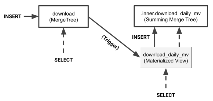
As the diagram shows, values from INSERT on the source table are transformed and applied to the target table. To populate the view all you do is insert values into the source table.
You can select from the target table as well as the materialized view. Selecting from the
materialized view passes through to the internal table that the view created automatically.

There’s one other important thing to notice from the diagram. The materialized view creates a private table with a special name to hold data. If you delete the materialized view by typing ‘DROP TABLE download_daily_mv’ the private table disappears. If you need to change the view you will need to drop it and recreate with new data.

Wrap-up

The example we just reviewed uses SummingMergeTree to create a view to add up daily user downloads. We used standard SQL syntax on the SELECT from the materialized view. This is a special capability of the SummingMergeTree engine and only works for sums and counts. For other types of aggregates we need to use a different approach.

Also, our example used the POPULATE keyword to publish existing table data into the private target table created by the view. If new INSERT rows arrive while the view is being filled ClickHouse will miss them. This limitation is easy to work around when you are the only person using a data set but problematic for production systems that constantly load data. Also, the private table goes away when the view is dropped. That makes it difficult to alter the view to accommodate schema changes in the source table.

In the next article we will show how to create materialized views that compute other kinds of aggregates like averages or max/min. We’ll also show how to define the target table explicitly and load data into it manually using our own SQL statements. We’ll touch briefly on schema migration as well. Meanwhile, we hope you have enjoyed this brief introduction and found the examples useful.

Get in touch with ClickHouse experts.

Get in touch with ClickHouse experts.

ClickHouse Materialized Views Illuminated, Part 1

How Materialized Views Work: Computing Sums

Wrap-up

Read part 2