ClickHouse® Aggregation Fun, Part 2: Exploring and Fixing Performance

The previous article in our series on aggregation explained how ClickHouse data warehouses collect aggregates using parallel processing followed by a merge to assemble final results. It also introduced system.query_log as well as server trace and debug messages. These are important tools to understand aggregation behavior.
In this second article we will apply our new knowledge to explore the performance of actual queries, so that we can understand some of the trade-offs around time and resource usage. We finish up with a list of practical tips to make aggregation even faster and more cost-efficient.
Exploring Aggregation Performance
Let’s look at aggregation in detail and test performance using example queries. We’ll vary three different aspects: GROUP BY keys, complexity of the aggregate function, and number of threads used in the scan. By keeping the examples relatively simple, we can more easily understand the trade-offs around aggregation.
Effect of values in the GROUP BY
Our original sample query had a few dozen GROUP BY values. Referring back to the hash tables used to hold results from scans, this means that such hash tables have a small number of keys. What if we run the same query with a different GROUP BY that generates far more values. Does the larger number of keys make a difference in the resources or speed of aggregation?
This is easy to test. First, let’s rerun our sample query followed by another that has a different GROUP BY.
SET max_untracked_memory = 1
-- #1
SELECT Carrier, avg(DepDelay) AS Delay
FROM ontime
GROUP BY Carrier
ORDER BY Delay DESC LIMIT 3
;
-- #2
SELECT Carrier, FlightDate, avg(DepDelay) AS Delay
FROM ontime
GROUP BY Carrier, FlightDate
ORDER BY Delay DESC LIMIT 314
If we now check the query speed and memory in system.query_log we see the following.
┌───────────€event_time─┬───€secs─┬─memory────┬─threads─┬─query───────────────┐
│ 2022-03-15 11:09:34 │ 0.725 │ 33.96 MiB │ 4       │ -- #2SELECT Carrier │
│ 2022-03-15 11:09:33 │ 0.831 │ 10.46 MiB │ 4       │ -- #1SELECT Carrier │
└────────────────────┴───────┴───────────┴─────────┴──────────────────────┘
There is a substantial difference in the amount of memory used by the second query. Having more keys takes up more RAM, at least in this case. What was the difference in the number of keys that caused this? We can find out using the following query. The handy uniqExact() aggregate counts the number of unique occurrences of values in rows.
SELECT
    uniqExact(Carrier),
    uniqExact(Carrier, FlightDate)
FROM ontime
FORMAT Vertical
Row 1:
───────€
uniqExact(Carrier):             35
uniqExact(Carrier, FlightDate): 169368
Our first query had 35 GROUP BY keys. Our second query had to handle 169,368 keys.
Before leaving this example, it’s worth noting that the second query is consistently about 15% faster than the first. That is surprising, because you might think that more GROUP BY keys means more work. As we explained elsewhere, ClickHouse picks different aggregation methods as well as different hash table configurations depending on the number and type of GROUP BY keys. They in turn vary in efficiency.
How do we know?
We can enable trace logging using the clickhouse-client –send_logs_message=’trace’ option, then look carefully at the messages. (See the previous article for instructions on how to do this.) It shows the time for scan threads to complete and also indicates the aggregation method. Here are a couple of typical messages from one of the threads in the second query.
[chi-clickhouse101-clickhouse101-0-0-0] 2022.03.28 14:23:15.311284 [ 1887 ] {92d8506c-ae7c-4d01-84b6-3c927ed1d6a5} <Trace> Aggregator: Aggregation method: keys32

…
[chi-clickhouse101-clickhouse101-0-0-0] 2022.03.28 14:23:16.007341 [ 1887 ] {92d8506c-ae7c-4d01-84b6-3c927ed1d6a5} <Debug> AggregatingTransform: Aggregated. 48020348 to 42056 rows (from 366.37 MiB) in 0.698374248 sec. (68760192.887 rows/sec., 524.61 MiB/sec.)
The scan threads run faster in the second case, which likely means that the chosen aggregation method and/or hash table implementation are simply quicker. To find out why we would need to dig into the code starting in src/Interpreters/Aggregator.h. There we could learn about keys32 and other aggregation methods. That investigation will have to wait for another blog article.
Effect of different aggregate functions
The avg() function is very simple and uses relatively little memory–basically a couple of integers for each partial aggregate it creates. What happens if we use a more complex function?
The uniqExact() function is a good one to try out. This aggregate stores a hash table containing values it sees in blocks and then merges them to get a final answer. We can hypothesize the hash tables will take more RAM to store and will be slower as well. Let’s look! We’ll run the following queries with both small and large numbers of GROUP BY keys.
SET max_untracked_memory = 1
SELECT Carrier, avg(DepDelay) AS Delay, uniqExact(TailNum) AS Aircraft
FROM ontime
GROUP BY Carrier ORDER BY Delay DESC
LIMIT 3
-- #2
SELECT Carrier, FlightDate, avg(DepDelay) AS Delay,
  uniqExact(TailNum) AS Aircraft
FROM ontime
GROUP BY Carrier, FlightDate ORDER BY Delay DESC
LIMIT 3
When we check the query performance in system.query_log we see the following results.
┌───────────€event_time─┬───€secs─┬─memory────┬─threads─┬─query────────────────┐
│ 2022-03-15 12:19:08 │ 3.324 │ 2.41 GiB  │ 4       │ -- #2SELECT Carrier  │
│ 2022-03-15 12:19:04 │ 2.657 │ 21.57 MiB │ 4       │ -- #1SELECT Carrier  │
. . .
There’s definitely a difference in execution time from adding this new aggregate, but that’s not really surprising. What’s more interesting is the increase in RAM. With a small number of keys it’s not very much: 21.57MiB compared to 10.46Mib in our original sample query.
However, the RAM usage explodes with more GROUP BY keys. This makes sense if you think about the query, which is asking for the exact count of airline tail numbers (i.e., the aircraft) that made flights in each group. Adding FlightDate to the GROUP BY means that the same aircraft are counted many more times, which means they have to be kept around in hash tables until ClickHouse can merge and do the final count.
Since we’re looking at explosive growth, let’s try one more query. The groupArray() function is a powerful aggregate unique to ClickHouse that collects column values within the group into an array. We hypothesize that it will use even more memory than uniqExact. That’s because it will hold all values and not just those we count.
And here is the query followed by the query log statistics.
SELECT Carrier, FlightDate, avg(DepDelay) AS Delay,
  length(groupArray(TailNum)) AS TailArrayLen
FROM ontime
GROUP BY Carrier, FlightDate ORDER BY Delay DESC
LIMIT 3
┌───────────€event_time─┬───€secs─┬─memory───┬─threads─┬─query───────────────┐
│ 2022-03-15 21:28:51 │ 2.957 │ 5.66 GiB │ 4       │ -- #3SELECT Carrier │
└────────────────────┴───────┴──────────┴─────────┴──────────────────────┘
As expected this takes even more memory than uniqExact: 5.66GiB. ClickHouse will by default terminate queries that use more than 10GiB, so this is approaching a problematic level. Notice, however, that all of these are still pretty fast given we’re scanning almost 200M rows. As before, there are variations in performance due to ClickHouse picking different aggregation methods and hash table implementations in each case.
Effect of the number of execution threads
For our last investigation we’ll look into the effect of threads. We can control the number of threads in the scan phase using max_threads. We’ll run the same query three times as follows:
SET max_untracked_memory = 1
SET max_threads = 1
SELECT Origin, FlightDate, avg(DepDelay) AS Delay,
  uniqExact(TailNum) AS Aircraft
FROM ontime
WHERE Carrier='WN'
GROUP BY Origin, FlightDate ORDER BY Delay DESC
LIMIT 3
SET max_threads = 2
(same query)
SET max_threads = 4
(same query)
OK, let’s look at the resulting memory usage. I added comments to make it easier to tell which query was which.
┌───────────€event_time─┬───€secs─┬─memory───┬─threads─┬─query───────────────┐
│ 2022-03-15 22:12:02 │  0.86 │ 1.71 GiB │ 8       │ -- #8SELECT Origin, │
│ 2022-03-15 22:12:01 │ 1.285 │ 1.72 GiB │ 4       │ -- #4SELECT Origin, │
│ 2022-03-15 22:11:59 │ 2.325 │ 1.75 GiB │ 2       │ -- #2SELECT Origin, │
│ 2022-03-15 22:11:56 │ 4.408 │ 1.91 GiB │ 1       │ -- #1SELECT Origin, │
. . .
It’s easier to understand the results if we put them in a graph.
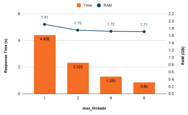
Adding threads significantly increases aggregation query speed up to a point, which in this case is 4 threads. At some point the scans stop speeding up with more threads–that’s the case here between 4 and 8 threads. Interestingly, ClickHouse parallelizes the merge operation after the scan runs. If you examine debug level messages carefully, you’ll see this part of query execution speed up as well.
Adding more threads affects memory usage, but perhaps not as you might think. In this case we use somewhat less RAM to process the query when there are more threads.
Practical tips to improve aggregation performance
We’ve looked in detail at aggregation response time and memory usage, which are two big considerations in production ClickHous implementations. In this final section we’ll summarize practical ways to improve both.
Make aggregation faster
There are a number of ways to make queries with aggregates go faster. Here are the main recommendations.
Remove or exchange complex aggregate functions
Using uniqExact to count occurrences? Try uniq instead. It’s faster at the cost of less precision in the answer. ClickHouse also has specific functions that can replace costly aggregation with a more specific implementation. If you are crunching data on website visitors to compute conversion rates, try windowFunnel.
Reduce values in GROUP BY
Processing large numbers of GROUP BY keys can add time to aggregation. Group by fewer items if possible.
Increase parallelization using max_threads
Increasing max_threads can result in close to linear response time improvements, though eventually adding new threads no longer increases throughput. At that point the cores you are adding are wasted.
Reduce processing in the initial scan with deferred joins
If you are joining against data it may be better to defer the join until after aggregation is complete. Here’s an example. ClickHouse will run the subquery first, then join the result with table airports.
SELECT Dest, airports.Name Name, c Flights, ad Delay
FROM
(
 SELECT Dest, count(*) c, avg(ArrDelayMinutes) ad
  FROM ontime
   GROUP BY Dest HAVING c > 100000
     ORDER BY ad DESC LIMIT 10
) a
LEFT JOIN airports ON IATA = Dest
If we join the tables directly, ClickHouse will join rows during the main scan, which requires extra CPU. Instead, we just join on 10 rows at the end after the subquery finishes. It greatly reduces the amount of processing time required.
This approach can also save memory but the effect probably may not be noticeable unless you add a lot of columns to the results. The example adds a single value per GROUP BY key, which is simply not very large in the grand scheme of things.
Round up the usual suspects
Following up on the previous point, any query runs faster if you process less data. Filter out unneeded rows, drop unneeded columns entirely, and all that good stuff.
Use materialized views
Materialized views pre-aggregate data to serve common use cases. In the best case they can reduce query response time by a factor of 1000x or more, simply by reducing the amount of data you need to scan. We’ve written extensively on materialized views in the Altinity Blog. They are one of the outstanding contributions to data management in the ClickHouse project.
Use memory more efficiently
Use materialized views (again)
Did we mention they save memory? A materialized view that pre-aggregates second-based measurements to hours, for example, can reduce enormously the size and number of partial aggregates ClickHouse drags around during the initial scan. Materialized views normally also use far less space in external storage.
Remove or exchange memory-intensive aggregate functions
Functions like max, min, and avg are very parsimonious with memory. Functions like uniqExact by contrast are memory hogs. To get an idea of the memory usage across functions to count unique occurrences, have a look at this Altinity Knowledge Base article.
Reduce number of keys in GROUP BY
Aggregates that record large numbers of items per block in partial aggregates can explode memory usage as the number of keys increases. Arrays can be a particular offender as we showed. If you can’t reduce the number of keys in the GROUP BY, another option is to use a materialized view to pre-aggregate for particular GROUP BY combinations.
Just give up, take one
Some queries take a lot of memory, and that’s how it goes. Raise the limits so they can run. ClickHouse memory limits are controlled by the following parameters, which you can alter at the system level or in user profiles (depending on the setting).
- max_memory_usage – Maximum bytes of memory for a single query. The default is 10GiB which is enough for most purposes but maybe not yours.
- max_memory_usage_for_user – Maximum bytes of all queries for a single user at a single point in time. Default is unlimited.
- max_server_memory_usage – Maximum memory for the entire ClickHouse server. Defaults to 90% of available RAM.
Just give up, take two
If all else fails, you can dump partial aggregates to external storage. Use the max_bytes_before_external_group_by setting. The standard recommendation is to set it at 50% of max_memory_usage. This ensures that you won’t run out in the merge phase.
Don’t take anything for granted
Test everything! Aggregation behavior seems complex, but you can figure it out. Use simple examples (if possible) and large datasets for your tests. In our experience at Altinity, it is usually possible to speed up queries, often significantly. Make hypotheses and test them. You’ll encounter surprises. Many of them will be good ones.
Conclusion
Aggregation is the fundamental operation in data warehouses to extract meaning from big data. ClickHouse aggregation is like a high-performance race car. It’s extremely fast, but you need training to win races. Do it right and you’ll get results in fractions of a second. Do it wrong and your queries will be slow or run out of memory.
In this two-part series we have covered how aggregation works, shown simple tools to check performance, and explored aggregation performance. I hope this article gets you closer to being a top-notch race car driver. If you have more questions about aggregation don’t hesitate to contact us at Altinity. You can use the Contact Us form, join our Slack Workspace, or send email to info@altinity.com. Meanwhile, have fun with ClickHouse aggregation!
ClickHouse® is a registered trademark of ClickHouse, Inc.; Altinity is not affiliated with or associated with ClickHouse, Inc.