ClickHouse® Aggregation Fun, Part 1: Internals and Handy Tools

Summarizing data into a digestible form is a key capability of analytic databases. Humans can’t conclude much from a list of billions of web page visits. However, we can easily understand that the average visit lasted 32 seconds this month, up from 25 seconds the previous month. In ClickHouse we call such summarization aggregation. It’s a fundamental way to grasp meaning from large datasets.
In this blog series we’ll explore how aggregation works in ClickHouse, how you can measure its performance, and how to make it faster and more efficient. We’ll use simple examples for readability, but the principles they show apply to far more complex queries.
The examples that follow use ClickHouse version 22.1.3.7 running on Altinity.Cloud. We will be using airline ontime data from the US Bureau of Transportation. There are approximately 197M rows in the table ontime. Each row represents a flight by a commercial aircraft.
How does an aggregation query work?
Let’s use a simple example to show how ClickHouse handles aggregation internally. Here’s a query to find the average departure delay for US airlines. It sorts the results in descending order and returns the three airlines with the longest average delay:
SELECT Carrier, avg(DepDelay) AS Delay
FROM ontime
GROUP BY Carrier
ORDER BY Delay DESC LIMIT 3
. . .
┌─Carrier─┬───────────────€Delay─┐
│ B6      │ 12.058290698785067 │
│ EV      │ 12.035012037703922 │
│ NK      │ 10.437692933474269 │
└────────┴─────────────────────┘
On my single cloud host, this query returns in around 0.75 seconds. It reads the full dataset, i.e., 197M rows to get this answer, which is pretty quick. So, what’s going inside ClickHouse? Here’s a picture that illustrates the query processing flow.
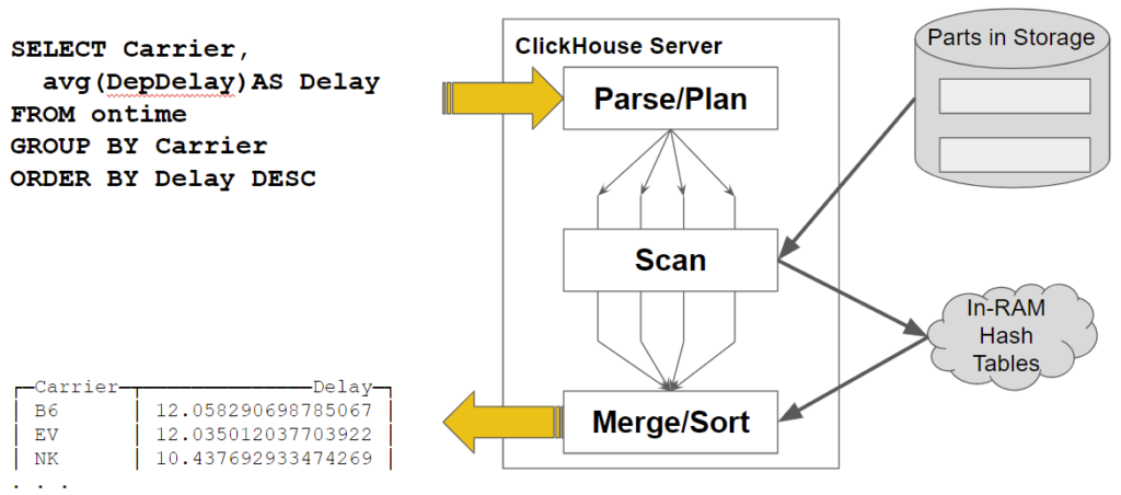
Let’s focus on two important features of processing aggregates that occur while scanning data.
- Query processing is parallelized. ClickHouse allocates multiple threads – four in this example – that independently read different table parts and blocks of data within them. They read the data and perform initial aggregation on the fly.
- Aggregates are accumulated in hash tables. There is a key for each GROUP BY value.
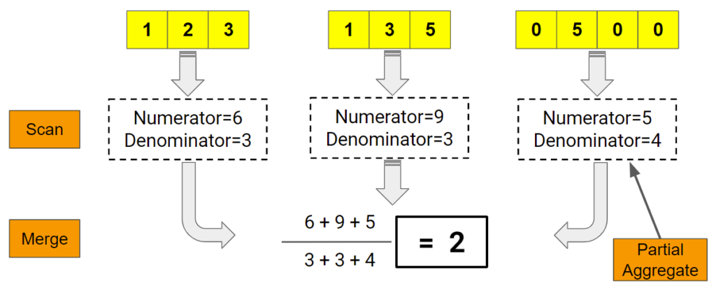
Once the scan ends, there is a final step to merge all the aggregates and sort them. Which brings up the next question. How does ClickHouse compute aggregates in parallel? Here’s a picture that shows how it works.
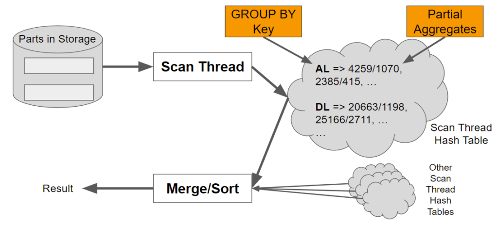
This leads to a final question. How does ClickHouse collect and store partial aggregates before merging? As we just mentioned, the answer is hash tables, where the key corresponds to the GROUP BY value and the partial aggregates are stored as lists associated with each key. Here’s another picture to illustrate.
ClickHouse aggregation is actually more sophisticated (and faster) than the above picture indicates.
First, ClickHouse picks different aggregation methods as well as different hash table configurations depending on the number and type of GROUP BY keys. The data structures and collection methods vary according to the data. This specialization ensures that the aggregation method accounts for differences in performance in different data types.
Second, ClickHouse aggregation is dynamic. ClickHouse starts with single-level hash tables, which are faster for small numbers of keys. As the number of stored keys increases, ClickHouse can shift automatically to two-level hash tables which operate faster. ClickHouse in effect adapts to actual data. It’s extremely fast without a lot of query planning overhead.
Speaking of query planning, there is an effort to add statistics that will allow ClickHouse to predict that it needs to go straight to two-level stables. (The pull request is here.) This is one of a number of ways to optimize aggregation performance that we may see implemented in future.
By the way, arranging aggregates into queues organized by keys and then merging the queue contents might sound familiar. You may have heard about MapReduce. It was the subject of a famous paper by Jeff Dean and Sanjay Ghemawat that contributed to the development of Hadoop. Data warehouses actually used this technique for many years before Hadoop made it widely popular.
Tools to measure aggregation performance
Now that we have looked into how aggregation works, it’s pretty obvious that there are some interesting issues related to aggregates. We need tools to understand query speed, memory used, and other characteristics. We also need a way to peek under the covers of query processing to look carefully at aggregation details.
Using system.query_log
Fortunately the system.query_log table has exactly the information needed to assess aggregate performance. It’s enabled by default when you install ClickHouse. Here’s a simple query to find out the time and memory required for our sample SQL, which appears third in the list.
SELECT
    event_time, query_duration_ms / 1000 AS secs,
    formatReadableSize(memory_usage) AS memory,
    Settings['max_threads'] AS threads,
    substring(query, 1, 20) AS query
FROM system.query_log AS ql
WHERE (user = 'default') AND (type = 'QueryFinish')
ORDER BY event_time DESC
LIMIT 50

Query id: 94c00711-31cb-4280-8270-717ccf942748

┌───────────€event_time─┬───€secs─┬─memory───┬─threads─┬─query────────────────┐
│ 2022-03-14 13:30:03 │ 0.007 │ 0.00 B   │ 4       │ select event_time, q │
│ 2022-03-14 13:23:52 │ 0.032 │ 0.00 B   │ 4       │ select event_time, q │
│ 2022-03-14 13:23:40 │ 2.023 │ 0.00 B   │ 4       │ SELECT Carrier, avg( │
│ 2022-03-14 13:23:20 │ 0.002 │ 0.00 B   │ 4       │ SELECT message FROM  │
│ 2022-03-14 13:23:20 │ 0.061 │ 4.24 MiB │ 4       │ SELECT DISTINCT arra │
. . .
The system.query_log table is quite versatile but we’ll concentrate on a couple of key columns. First, there are multiple events logged per query. The event name is in the type column. We’ll focus on the QueryFinish event type, as it shows the full statistics for the query.
Second, the query_duration_ms and memory_usage columns show the duration and memory usage of the query, respectively. They are easy to interpret, but you may be surprised that many queries seem to use 0 bytes of RAM. This obviously can’t be possible.
What’s happening is simple. ClickHouse ignores thread memory values that are below the value of max_untracked_memory, which defaults to 4,194,304. We can find out the memory in use for our query by setting the value to something low like 1 byte. Here’s an example.
SET max_untracked_memory = 1

SELECT Carrier, avg(DepDelay) AS Delay
FROM ontime
GROUP BY Carrier
ORDER BY Delay DESC LIMIT 3

SELECT
    event_time, query_duration_ms / 1000 AS secs,
    formatReadableSize(memory_usage) AS memory,
    Settings['max_threads'] AS threads,
    substring(query, 1, 20) AS query
FROM system.query_log
WHERE (user = 'default') AND (type = 'QueryFinish')
ORDER BY event_time DESC
LIMIT 50

┌───────────€event_time─┬───€secs─┬─memory───┬─threads─┬─query────────────────┐
│ 2022-03-14 13:35:09 │  0.85 │ 8.40 MiB │ 4       │ SELECT Carrier, avg( │
. . .
Averages use relatively little memory because the aggregation is simple. More complex aggregations use far more memory, so you won’t need to adjust max_untracked_memory in those cases to get an idea of the memory in use.
There are many other useful columns in system.query_log. However, the simple query shown above already provides abundant information that will enable us to measure trade-offs in aggregation processing. Inspect the others at your leisure.
Enabling message logs for queries
Another important tool is ClickHouse server message logs. You can look at the message logs directly, direct them to the system.text_log table, or enable them within clickhouse-client using the send_message_logs property. Here’s how to enable trace messages to show the gory details of query processing, along with a couple of enticing messages to show what you can learn.
SET send_logs_level = 'trace'

SELECT Carrier, FlightDate, avg(DepDelay) AS Delay
FROM ontime
GROUP BY Carrier, FlightDate
ORDER BY Delay DESC LIMIT 3
[chi-clickhouse101-clickhouse101-0-0-0] 2022.03.16 22:23:39.802817 [ 485 ] {287891a8-d444-4d43-a96a-ca7aa5cd6ff5} <Debug> executeQuery: (from xx.xxx.xx.xx:43802, user: default) -- #2
 SELECT Carrier, FlightDate, avg(DepDelay) AS Delay FROM ontime GROUP BY Carrier, FlightDate ORDER BY Delay DESC LIMIT 3 ;
. . .
[chi-clickhouse101-clickhouse101-0-0-0] 2022.03.16 22:23:39.810727 [ 282 ] {287891a8-d444-4d43-a96a-ca7aa5cd6ff5} <Trace> Aggregator: Aggregation method: keys32
. . .
[chi-clickhouse101-clickhouse101-0-0-0] 2022.03.16 22:23:40.530650 [ 282 ] {287891a8-d444-4d43-a96a-ca7aa5cd6ff5} <Debug> AggregatingTransform: Aggregated. 50160884 to 42533 rows (from 382.70 MiB) in 0.721708392 sec. (69502980.090 rows/sec., 530.28 MiB/sec.)
Debug level output is sufficient to see timings on threads. If you want to see things like the aggregation method selected (for example keys32 as shown above), trace is your friend. It generates staggering amounts of output for large queries.
Conclusion of Part 1
In this first part we looked at ClickHouse aggregation internals to see how aggregation works. We also covered two basic tools to track aggregation behavior: the system.query_log table and ClickHouse debug and trace logs.
In the next part of this series we will put this knowledge to practical use. We will explore aggregation performance using specific examples, then give advice on how to boost execution speed while reducing resource consumption. Stay tuned!
ClickHouse® is a registered trademark of ClickHouse, Inc.; Altinity is not affiliated with or associated with ClickHouse, Inc.