Reading External Parquet Data from ClickHouse

ClickHouse support for Apache Parquet is outstanding. We blogged about it last year in “What’s Up With Parquet Performance in ClickHouse”. In this article, we will look at Parquet from a different perspective. Let’s say there is public Parquet data somewhere in the cloud. What is the best way to analyze it from ClickHouse?

Reading Public Blockchain Datasets from S3

There are multiple public datasets available on AWS. Among other treasures we find AWS public blockchain data. Two separate datasets are organized under two prefixes:

• s3://aws-public-blockchain/v1.0/btc/ for Bitcoin.
• s3://aws-public-blockchain/v1.0/eth/ for Etherium

Inside each prefix there are multiple Parquet files with following path patterns. Let’s take Bitcoin for example. 

• blocks/date={YYYY-MM-DD}/{id}.snappy.parquet
• transactions/date={YYYY-MM-DD}/{id}.snappy.parquet

Now let’s try to read those from ClickHouse. Of course, we could use the s3() table function in order to query files, or load into a table in ClickHouse for faster analysis. But let’s try something new today – an overlay database!

Overlay databases are a nice feature of ClickHouse. For example, one can define a database with MySQL engine that would connect to a MySQL server and expose all tables from a remote MySQL database as ClickHouse tables. ClickHouse then can run queries, insert data and so on – but using a remote MySQL server as a data source. Similar functionality is available for S3 buckets since ClickHouse version 23.7. For example, we may create database that connects to a public S3 bucket like this: 

CREATE DATABASE aws_public_blockchain
ENGINE = S3('s3://aws-public-blockchain/v1.0/btc/', NOSIGN)

Once created, we may access all files using SQL; we do not need to use the S3 table function anymore. For example, let’s try something very simple and check how many Parquet files represent Bitcoin blocks:

SELECT uniq(_path) from aws_public_blockchain."blocks/**.parquet"
┌─uniq(_path)─┐
│        5644 │
└─────────────┘

Note that the glob pattern is interpreted as a table name! If one is using ‘clickhouse-client’, or any other client that supports sessions, it is possible to make it even more explicit:

USE aws_public_blockchain
SELECT uniq(_path) from "blocks/**.parquet"

So there are more than 5600 files corresponding to blocks, one or two per day. This is different from our previous tests of ClickHouse with Parquet, when we usually took one file or a small number of files. And this difference is essential that we will see later.

Let’s continue exploring and look into the number of Bitcoin transactions:

SELECT uniq(_path), count()
FROM aws_public_blockchain."transactions/**.snappy.parquet"
┌─uniq(_path)─┬───count()─┐
│        5622 │ 978253085 │
└─────────────┴───────────┘
1 row in set. Elapsed: 35.582 sec. Processed 978.25 million rows, 0.00 B (27.49 million rows/s., 0.00 B/s.)
Peak memory usage: 1.70 GiB.

Almost 1 billion transactions already! It took over 30 seconds to get the result. Not super-fast, but given that it has to read at least the header of 5622 files, this is understandable. We can see it in profile events of the query as well:

┌─pe───────────────────────────────┐
│ ('S3ReadMicroseconds',868047843) │
│ ('S3ReadRequestsCount',6097)     │
│ ('S3ListObjects',6)              │
│ ('S3GetObject',6091)             │
└──────────────────────────────────┘

SELECT arrayJoin(ProfileEvents) AS pe
FROM system.query_log
WHERE event_date = today() AND pe.1 LIKE 'S3%'
  AND query_id = '22ce40b1-a7a3-43ea-8275-5f8026582f8f' 

You may also specify a custom marker by adding “SETTINGS log_comment='my_log_comment‘” at the end of the query. Here’s how to find the query with your comment value instead. 

SELECT arrayJoin(ProfileEvents) AS pe
FROM system.query_log
WHERE event_date = today() AND pe.1 LIKE 'S3%'
  AND log_comment = 'my_query_id' 

Now we can explore the structure of the data and run some queries:

SELECT *
FROM aws_public_blockchain."transactions/**.snappy.parquet"
LIMIT 1 FORMAT Vertical;

Row 1:
──────
hash:            4a5e1e4baab89f3a32518a88c31bc87f618f76673e2cc77ab2127b7afdeda33b
version:         1
size:            204
block_hash:      000000000019d6689c085ae165831e934ff763ae46a2a6c172b3f1b60a8ce26f
block_number:    0
virtual_size:    204
lock_time:       0
input_count:     0
output_count:    1
is_coinbase:     true
output_value:    50
outputs:         [(0,1,'04678afdb0fe5548271967f1a67130b7105cd6a828e03909a67962e0ea1f61deb649f6bc3f4cef38c4f35504e51ec112de5c384df7ba0b8d578a4c702b6bf11d5f OP_CHECKSIG','4104678afdb0fe5548271967f1a67130b7105cd6a828e03909a67962e0ea1f61deb649f6bc3f4cef38c4f35504e51ec112de5c384df7ba0b8d578a4c702b6bf11d5fac','pubkey',50)]
block_timestamp: 2009-01-03 18:15:05.000000000
date:            2009-01-03

So we can see column names and can guess data types easily. ClickHouse uses data type inference for Parquet, so we do not need to worry about type conversions. 

Let’s query the transaction volumes in 2024 aggregated by day:

SELECT date, count()
FROM aws_public_blockchain."transactions/**.snappy.parquet"
WHERE date>='2024-01-01'
GROUP BY date ORDER BY date

┌─date───────┬─count()─┐
│ 2024-01-01 │  657752 │
│ 2024-01-02 │  367319 │
│ 2024-01-03 │  502749 │
...
└────────────┴─────────┘

The query takes 30 seconds, since ClickHouse needs to check every Parquet file. That is quite inefficient. ClickHouse does not know how files are organized. But we do! So we can use the glob filter to select only 2024 files:

SELECT date, count()
FROM aws_public_blockchain."transactions/date=2024*/*.snappy.parquet"
WHERE date>='2024-01-01'
GROUP BY date ORDER BY date

Now it takes only 2 seconds! Finally we can use ClickHouse “play” interface (user:demo, password:demo) and plot the chart with the transaction amount. It shows a plausible weekly pattern:

SELECT toDateTime(date)::INT, sum(output_value)
FROM aws_public_blockchain."transactions/date=2024*/*.snappy.parquet"
WHERE date>='2024-01-01'
GROUP BY date ORDER BY date
FORMAT JSONCompactColumns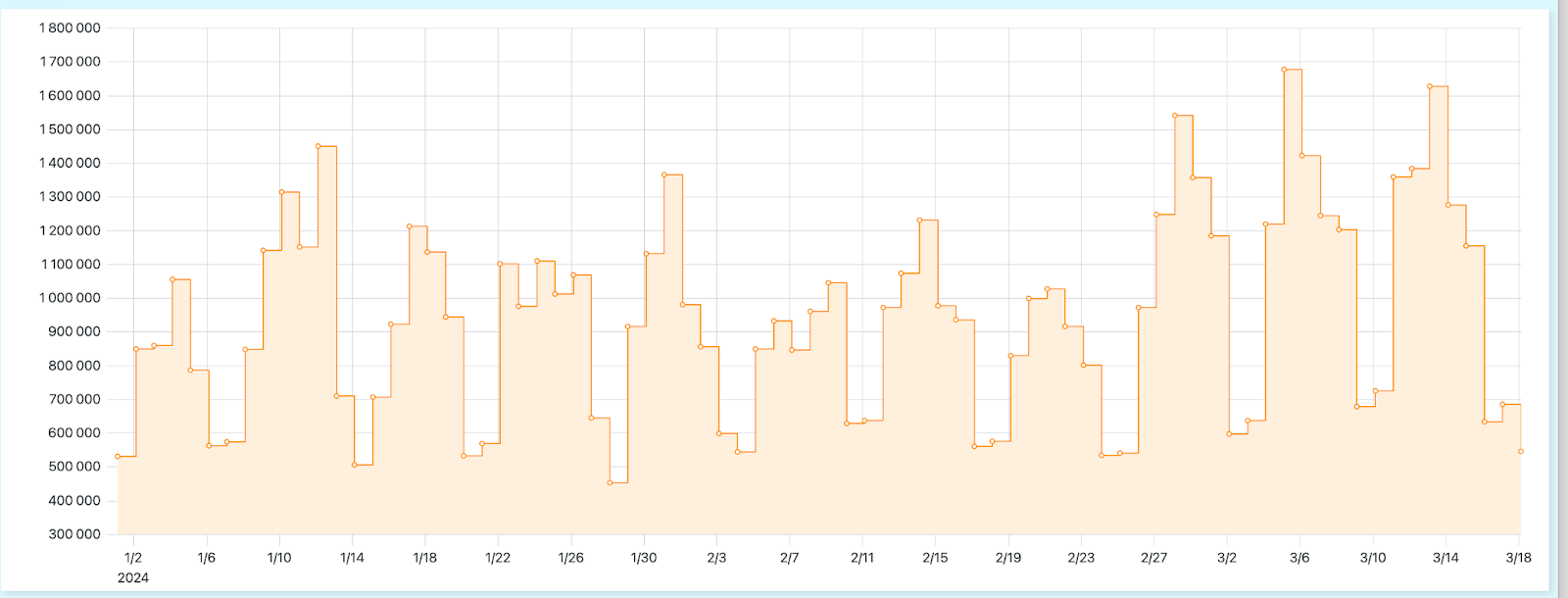

Since the data is public, you can play around with it and try other queries.

So working directly with external Parquet data is possible. It is even suitable for interactive analysis. However, the performance may be mediocre on datasets with a large number of Parquet files. This is usually the case for time ordered data. The 5000 thousand files in the bitcoin data are already an issue. In order to get good performance it is required to filter files using glob patterns, since ClickHouse can not pre-filter files by itself. We will get back to that point in a minute.

Reading Public Data from HTTP Servers

Not all datasets are organized as well as AWS samples. In academia, much data is still sitting on FTP servers. FTP is not a database friendly communication protocol, so is there a way to analyze such data without writing ETL jobs? The answer is “yes”, if the FTP server is open to the web using a basic HTTP server. With a little bit of help, ClickHouse can read HTML pages, extract references to Parquet files, and represent them as tables in ClickHouse. See details in the Appendix at the end of the article. 

Efficiency and Future Work

Knowing the organization of objects in the bucket is important when querying Bitcoin transactions, since it allows us to apply glob patterns as a filter. Otherwise, each query will have to inspect every single Parquet file even if it does not contain relevant data. ClickHouse can do it quite effectively, checking Parquet metadata, but still it requires a lot of network, data transfer and other overheads. When querying native MergeTree tables, ClickHouse can use indices and parts metadata stored in RAM or an internal catalog to skip reading unnecessary parts. With external Parquet data this is not yet possible.

There are several potential approaches to improve efficiency there. One path is to implement a special part type for ClickHouse, that would store data in Parquet instead of native ClickHouse format. The idea was proposed by Altinity in “Parquet part format for MergeTree RFC” while back. If implemented, it would open up a lot of interesting capabilities, including adopting external Parquet stores as read-only MergeTree tables. That requires a lot of work, though, so it was put on the shelf for now. It also does not address Parquet data written by programs other than ClickHouse.

Another approach is to use external catalogs that store data in Parquet, utilizing tools to organize metadata properly, but represent them using a different interface. ClickHouse supports three types of data lake catalogs: Apache Iceberg, DeltaLake and Apache Hudi. As usual, those are represented as table functions or table engines:

CREATE TABLE data_lake ENGINE = DeltaLake/Hudi/Iceberg(...)

When querying the data, predicates are pushed down to the data lake engine that is responsible for efficient query handling in this case. ClickHouse does this as well, filtering row groups without reading the data, but it can not do it across many files.

Finally, there could be improvements to ClickHouse itself. ClickHouse could cache the metadata of Parquet files in RAM, for example, and use it in order to filter Parquet files on an early query stage without hitting the remote storage. Since Parquet files are immutable, maintaining such a cache should be quite easy to do. Well, why don’t we make a simple prototype right now? Let’s try!

Parquet Metadata Cache Prototype

For the prototype purposes we will create a reverse index table that would map column ranges to file names or paths. For simplicity, we will use strings for all column types:

CREATE TABLE aws_public_blockchain_idx (
  path String,
  file String,
  column String,
  min_value String,
  max_value String
) Engine = MergeTree
PARTITION BY tuple()
ORDER BY (column, min_value)

In order to populate ranges, we will lean on the ClickHouse ability to read Parquet metadata. Parquet metadata is a part of the Parquet file, It contains column definitions plus internal statistics including min and max boundaries for every column. We can read it by specifying ParquetMetadata format in the s3() table function:

SELECT * FROM s3('s3://aws-public-blockchain/v1.0/btc/transactions/date=2009-01-03/part-00000-bdd84ab2-82e9-4a79-8212-7accd76815e8-c000.snappy.parquet', NOSIGN, 'ParquetMetadata') format PrettyJSONEachRow

Now, let’s extract min/max boundaries from a single Parquet file. Since there could be multiple row groups in one file, we need to aggregate across all of them:

SELECT _path, _file, column, min(min_value), max(max_value) FROM (
WITH arrayJoin(tupleElement(arrayJoin(row_groups), 'columns')) as row_groups_columns,
     tupleElement(row_groups_columns, 'statistics') as statistics
SELECT _path, _file,
        tupleElement(row_groups_columns, 'name') column,
        tupleElement(statistics, 'min') min_value,
        tupleElement(statistics, 'min') max_value
FROM s3('s3://aws-public-blockchain/v1.0/btc/transactions/date=2009-01-03/part-00000-bdd84ab2-82e9-4a79-8212-7accd76815e8-c000.snappy.parquet', NOSIGN, 'ParquetMetadata') 
)
GROUP BY _path, _file, column
format Vertical

A row of our improvised reverse index look like this:

Row 1:
──────
_path:          aws-public-blockchain/v1.0/btc/transactions/date=2009-01-03/part-00000-bdd84ab2-82e9-4a79-8212-7accd76815e8-c000.snappy.parquet
_file: part-00000-bdd84ab2-82e9-4a79-8212-7accd76815e8-c000.snappy.parquet
column:         value
min(min_value): 50.000000
max(max_value): 50.000000

Now we are ready to build an index for the entire dataset:

INSERT INTO aws_public_blockchain_idx
SELECT _path, _file, column, min(min_value), max(max_value) from (
WITH arrayJoin(tupleElement(arrayJoin(row_groups), 'columns')) as row_groups_columns
     tupleElement(row_groups_columns, 'statistics') as statistics
SELECT _path, _file,
        tupleElement(row_groups_columns, 'name') column,
        tupleElement(statistics, 'min') min_value,
        tupleElement(statistics, 'min') max_value
FROM s3('s3://aws-public-blockchain/v1.0/btc/transactions/**.snappy.parquet', NOSIGN, 'ParquetMetadata') 
)
GROUP BY _path, _file, column

The index contains 139K rows. Using this index, we can quickly find Parquet files that match query conditions. For example, let’s find all files for 2024.

SELECT path FROM aws_public_blockchain_idx
WHERE column='date' and toDateOrNull(min_value)>='2024-01-01'

That returns only 125 files out of 5600! Let’s try if we can use it in the query. In order to do it, we will add a filter to the virtual column ‘_path’:

SELECT date, count()
FROM aws_public_blockchain."transactions/**.snappy.parquet"
WHERE _path in (
     SELECT path FROM aws_public_blockchain_idx
      WHERE column='date' and toDateOrNull(min_value)>='2024-01-01')
  AND date >= '2024-01-01'
GROUP BY date ORDER BY date

78 rows in set. Elapsed: 61.714 sec. Processed 32.13 million rows, 645.16 MB (520.65 thousand rows/s., 10.45 MB/s.)
Peak memory usage: 8.60 MiB.

That works, but it takes 60 seconds! This is unexpected, so let’s try to figure out why. Here are profile events from the query above:

┌─pe──────────────────────────────┐
│ ('S3ReadMicroseconds',57323611) │
│ ('S3ReadRequestsCount',477)     │
│ ('S3ListObjects',6)             │
│ ('S3GetObject',471)             │
└─────────────────────────────────┘

Let’s compare to the query that uses glob instead of an index:

SELECT date, count()
FROM aws_public_blockchain."transactions/date=2024*/*.snappy.parquet"
WHERE date >= '2024-01-01'
GROUP BY date ORDER BY date

81 rows in set. Elapsed: 2.634 sec. Processed 33.05 million rows, 859.97 MB (12.55 million rows/s., 326.50 MB/s.)
Peak memory usage: 290.36 MiB.

┌─pe──────────────────────────────┐
│ ('S3ReadMicroseconds',66189599) │
│ ('S3ReadRequestsCount',631)     │
│ ('S3ListObjects',1)             │
│ ('S3GetObject',630)             │
└─────────────────────────────────┘

This is very interesting: the S3 read time is even slightly bigger, but the query is 30 times faster! Note also the memory usage – it is 33 times bigger as well. It looks like the reason is parallelization: when processing globs, ClickHouse loads every file in parallel using 32 threads. However, when _path filter is used, it processes paths sequentially in a single thread. 

Finally, let’s try to generate glob patterns explicitly using this very awkward query:

SELECT date, count()
FROM s3('s3://aws-public-blockchain/{' 
     || arrayStringConcat((SELECT arrayMap(p -> extract(p, 'aws-public-blockchain/(.*)'), groupArray(path)) 
                             FROM aws_public_blockchain_idx
                            WHERE column = 'date' AND toDateOrNull(min_value) >= '2024-01-01'), ',')
     || '}', NOSIGN, Parquet)
WHERE date >= '2024-01-01'
GROUP BY date ORDER BY date

┌─pe──────────────────────────────┐
│ ('S3ReadMicroseconds',57718386) │
│ ('S3ReadRequestsCount',517)     │
│ ('S3ListObjects',43)            │
│ ('S3GetObject',471)             │
│ ('S3Clients',1)                 │
└─────────────────────────────────┘

It also works, but it is still twice slower than a full scan taking around 60 seconds. Note the increased number of S3ListObject requests. Most probably this happens due to this ClickHouse bug. 

While the idea of the metadata index is tempting, it requires some ClickHouse server development to be done. Ideally, ClickHouse should process query conditions and use them in order to select proper Parquet files. Combined with overlay databases, it would enable ClickHouse to work much better with big external datasets.

Conclusion

ClickHouse can access external Parquet data using table functions like s3() or url(). The traditional approach is to use those for data import and export only. But in some cases, when there is no need or no possibility to store the data locally, ClickHouse can query external data efficiently enough for many applications. Overlay databases provide a convenient syntactic sugar when accessing S3 buckets. This does not work for not-so-well-structured file stores. Here, ClickHouse power comes into play, allowing us to parse HTML pages and query files directly from an HTTP server.

The efficiency of processing external data is a concern. While ClickHouse can use Parquet metadata for a single file, it can not work efficiently with a collection of files. Using globs somewhat helps, but it requires an understanding of file name patterns. Future improvements to ClickHouse may address this. If you are interested to participate in development of better Parquet support in ClickHouse  – join community efforts in doing so. The beauty of open source is that everybody can help. 

As the amount of data grows, it becomes essential to be able to process data close to where it is stored. The network costs and latencies may be substantial otherwise. Thanks to Clickhouse portability, it can be deployed as close to the data as needed. It can be any AWS, GCP or Azure region, or a private cloud. And if you are unsure how to do it properly – Altinity and our Altinity.Cloud platform for ClickHouse can help.

|——————————

Appendix: Reading Public Data from HTTP Servers

In this part, we will look how to load Parquet data from a generic HTTP server. Here is an example of open data from European Bioinformatics Institute:

http://ftp.ebi.ac.uk/pub/databases/opentargets/platform/23.12/output/etl/parquet/targets/

If you follow the link you will see the simple HTML page with links to Parquet files.

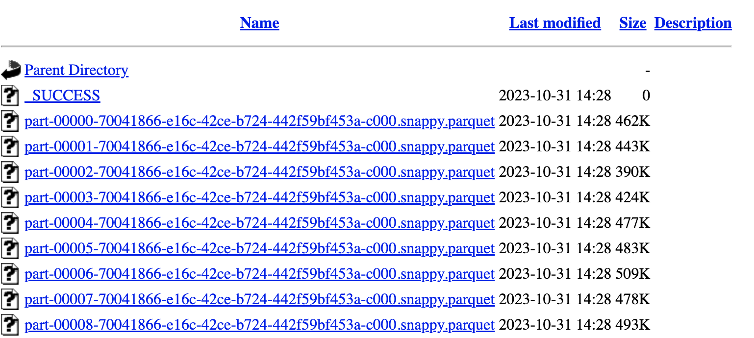
We can take any link and use the url() table function in order to retrieve the Parquet file:

SELECT * FROM url('http://ftp.ebi.ac.uk/pub/databases/opentargets/platform/23.12/output/etl/parquet/targets/part-00000-70041866-e16c-42ce-b724-442f59bf453a-c000.snappy.parquet') LIMIT 1 FORMAT Vertical

Row 1:
──────
id:                   ENSG00000020219
approvedSymbol:       CCT8L1P
biotype:              processed_pseudogene
transcriptIds:        ['ENST00000465400']
canonicalTranscript:  ('ENST00000465400','7',152445477,152447150,'+')
canonicalExons:       ['152445477','152447150']
genomicLocation:      ('7',152445477,152447150,1)
alternativeGenes:     []
approvedName:         chaperonin containing TCP1 subunit 8 like 1, pseudogene

So, we can query or load a single file. But what about all files? How to query them all together? The plan is the following:

1. Load HTML page
2. Parse HTML page and extract file names
3. Create URL table for every file
4. Create a merge table overlay for all files!

So let’s start with HTML. We will use the url() table function in order to load the HTML page!

SELECT * from url('http://ftp.ebi.ac.uk/pub/databases/opentargets/platform/23.12/output/etl/parquet/targets/', TSVRaw)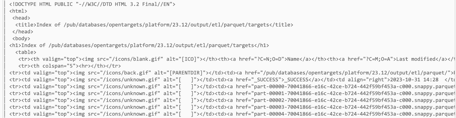

TSVRaw format is used in order to split output into rows without any extra processing. We can see ‘href’ elements pointing to files. It is easy then to extract them using a regular expression:

SELECT DISTINCT extract(r, 'href="([^"]+\\.parquet)"') AS file_parquet
FROM url('http://ftp.ebi.ac.uk/pub/databases/opentargets/platform/23.12/output/etl/parquet/targets/', TSVRaw, 'r String') WHERE file_parquet != ''

┌─file_parquet─────────────────────────────────────────────
──────────┐
│ part-00000-70041866-e16c-42ce-b724-442f59bf453a-c000.snappy.parquet │
│ part-00001-70041866-e16c-42ce-b724-442f59bf453a-c000.snappy.parquet │
│ part-00002-70041866-e16c-42ce-b724-442f59bf453a-c000.snappy.parquet │
...

Now we have a list of files, and for every file we will create a separate url() engine table:

WITH files AS (select distinct extract(r, 'href="([^"]+\.parquet)"') file_parquet
FROM url('http://ftp.ebi.ac.uk/pub/databases/opentargets/platform/23.12/output/etl/parquet/targets/', TSVRaw, 'r String')
WHERE file_parquet != '')
SELECT 'CREATE TABLE target_all."' || file_parquet || '" Engine = URL(\'http://ftp.ebi.ac.uk/pub/databases/opentargets/platform/23.12/output/etl/parquet/targets/' || file_parquet || '\');'
FROM files

The query above is a generator. It generates a set of CREATE TABLE statements that needs to be executed separately:

CREATE TABLE target_all."part-00000-70041866-e16c-42ce-b724-442f59bf453a-c000.snappy.parquet" ENGINE = URL('http://ftp.ebi.ac.uk/pub/databases/opentargets/platform/23.12/output/etl/parquet/targets/part-00000-70041866-e16c-42ce-b724-442f59bf453a-c000.snappy.parquet');

CREATE TABLE target_all."part-00001-70041866-e16c-42ce-b724-442f59bf453a-c000.snappy.parquet" Engine = URL('http://ftp.ebi.ac.uk/pub/databases/opentargets/platform/23.12/output/etl/parquet/targets/part-00001-70041866-e16c-42ce-b724-442f59bf453a-c000.snappy.parquet');
...

Once tables are created, we may query data using merge() table function:

SELECT count() FROM merge('target_all', '.*parquet')

┌─count()─┐
│   62733 │
└─────────┘

Or create an overlay table:

CREATE TABLE target_all.targets as merge('target_all', '.*parquet')

Finally, we are ready to do some quick analysis on the data, e.g. find top gene biotypes:

SELECT biotype, count() FROM target_all.targets
GROUP BY 1 ORDER BY 2 DESC LIMIT 10

It only takes 10 seconds to see the result:

┌─biotype────────────────────────────┬─count()─┐
│ protein_coding                     │   20073 │
│ lncRNA                             │   18866 │
│ processed_pseudogene               │   10146 │
│ unprocessed_pseudogene             │    2609 │
│ misc_RNA                           │    2212 │
│ snRNA                              │    1901 │
│ miRNA                              │    1879 │
│                                    │    1056 │
│ transcribed_unprocessed_pseudogene │     961 │
│ snoRNA                             │     942 │
└────────────────────────────────────┴─────────┘

Not surprisingly, most genes are used for protein coding.