Database comparison [2020]: ClickHouse vs Redshift for FinTech

Readers of this blog know we love fast analytic applications. As we demonstrated in a previous article, ClickHouse outperformed Redshift on a NYC Taxi rides benchmark. The benchmark queries are very simple, however.

Real life use cases often require much more complex data processing. It is especially true for fintech applications.

We have explored ClickHouse use cases in fintech before, for example at a Percona Live 2018 talk. And last year Prerak Sanghvi from Prooftrading showed that ClickHouse beats MemSQL as a backend for algorithmic trading.

This time Paris based startup Opensee, a capital market fintech, suggested an interesting risk management use case they solved leveraging Clickhouse.

Opensee empowers financial institutions to extract and analyze billions of data rows in real time for Front-office Risk and P&L, Market and Credit Risk, Liquidity Management, Market Data etc. Their solution extensively uses ClickHouse for all sorts of aggregations and statistics required for risk computation.

We took the challenge and looked at it from different angles, showcasing how ClickHouse can adapt to specific use cases unlike other traditional SQL databases such as Redshift.

For impatient readers, here is the punch line. ClickHouse SQL extensions, arrays, in particular, allow it to solve the business use case up to 100 times more efficiently than Redshift at 1/6th the cost. We know that ClickHouse is fast, but we were a bit surprised by these research results.

Use Case: FinTech Risk Management

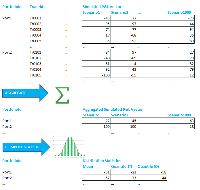
Let’s consider a financial cube typically used for risk management purposes, for example profit and loss (P&L) or mark-to-market values under stressed market conditions. Such cubes may be quite big, containing hundreds of dimensions of different data types. Every record is associated with a vector of measurements. The vectors are quite long, e.g. 1000 elements.

Typically this cube will store for every financial trade and for every date, a vector of P&L values representing different market scenarios (computed using historical based simulations or a Monte Carlo simulation).

The various dimensions represent some of the trade attributes (such as portfolios hierarchy, product type, or counterparty) which are required as potential aggregation levels or filtering criteria when performing the risk computation.

The typical question that we may pose with this data is the following. What is the maximum loss in statistical terms that we may expect for each of my portfolios? These metrics are usually referred to as Value-at-Risk, Expected Shortfall, etc., in the risk management terminology.

First, we aggregate the P&L vectors for each portfolio in order to get a probability distribution. Then we can apply different statistical methods.

For example, if we want to compute the maximum loss at a 95% confidence interval (Value-at-Risk), we can sort the resulting vectors of 1000 elements and take the 50th element in order to get 5% quantile.

Below is the diagram to illustrate the process:

Since such data is usually private, we have generated it using a tool provided by Opensee. It produces a sample dataset with 100 dimensions of different types represented as int0-int33, dttime0-dttime32, str0-str32 respectively, and P&L vectors of 1000 elements.

For benchmarking we use the same setup as in the previous article: ClickHouse 20.6.4.44 running in Kubernetes within a m5.8xlarge AWS instance (32 vCPUs 120GB RAM, $1.54 per hour), and Redshift on two dc2.8xlarge instances (2 x 32 vCPUs 244GB RAM, $9.6 per hour).

The dataset is small, and the data is cached after the first run, so we are measuring pure computational capabilities of both analytical DBMS.

ClickHouse Schema

The most natural way to represent vectors in ClickHouse is arrays. ClickHouse has very well developed functionality around arrays, including aggregate functions on arrays, lambda expressions and more. Arrays allow you to avoid extra tables and joins when there is a 1-to-N relationship between entities.

In our case every cube cell ‘stores’ a vector of values, so we can have a reference to a separate table, or store the vector in an array. We will start with the array approach, but will later look into the separate table as well, since we need to do it for the Redshift schema anyway.

Thus we have the following schema in ClickHouse (please refer to the repository for a complete set of schema and query examples):

CREATE TABLE factTable (
  index Int64,
  int0 Int64, ... , int33 Int64,
  dttime0 DateTime, ... , dttime32 DateTime,
  str0 String, ... , str32 String,
  arrFloat Array(Float32),
  partition Int6
) ENGINE = MergeTree
PARTITION BY partition
ORDER BY tuple()

The table has following columns:

Index — unique row ID
Int0-int33, dttime0-dttime32, str0-str32 are dimension columns
arrFloat — P&L vector
partition — partitioning column, usually it is a day

There is no primary key and ordering, as this is just a cube.

We have loaded the table with dataset_gen.py. It generated 1.72M rows taking 6.8GB of storage.

Once it is ready, let’s look at test queries suggested by our friends from Opensee.

Queries

The basic question that we want to answer is the maximum loss for a portfolio with a given confidence level. ClickHouse can aggregate arrays, summing elements position by position with the ‘sumForEach’ function.

This is an aggregate function that takes an array column as an argument and results in an array, where the 1st element is a sum of 1st elements of all arrays in the group, 2nd element is a sum of 2nd elements of all arrays in the group and so on.

In order to calculate quantiles for values stored in an array of a known size we may just sort an array and take a corresponding element. Since we have 1000 elements, 5% quantile is the 50th element.

Q1. Maximum loss with a 95% confidence (5% quantile) for a single dimension.

SELECT
    str0,
    arraySort(sumForEach(arrFloat))[50] AS arr1
FROM factTable
GROUP BY str0

Q2. Maximum loss with a 95% confidence (5% quantile) for a group of 6 dimensions.

SELECT
    str0, str1, int10, int11, dttime10, dttime11,
    arraySort(sumForEach(arrFloat))[50] AS arr1
FROM factTable
GROUP BY
    str0, str1, int10, int11, dttime10, dttime11

Q3. Maximum loss with a 95% confidence (5% quantile) for a group of 12 dimensions.

SELECT
    str0, str1, str2, str3, int10, int11, int12, int13, dttime10, dttime11, dttime12, dttime13,
    arraySort(sumForEach(arrFloat))[50] AS arr1
FROM factTable
GROUP BY
    str0, str1, str2, str3, int10, int11, int12, int13, dttime10, dttime11, dttime12, dttime13

Q4. Query with a filter and unfold results to rows.

SELECT
    str0, num, pl
FROM (
    SELECT str0, 
           sumForEach(arrFloat) AS arr1
    FROM factTable
    WHERE str1 = 'KzORBHFRuFFOQm'
    GROUP BY str0
)
ARRAY JOIN
    arr1 AS pl,
    arrayEnumerate(arr1) AS num

Note the ARRAY JOIN clause in the last query. It is used in order to unfold multiple arrays of the same size to rows. It is often used together with the arrayEnumerate function that generates a list of indexes (1,2,3 … ) for a given array.

ClickHouse can calculate quantities on arrays directly as well, so Q1 can be executed as follows:

SELECT
    str0,
    arrayReduce('quantilesExact(0.05)',sumForEach(arrFloat)) AS arr1
FROM factTable
GROUP BY str0

Here we are using the arrayReduce function that comes from functional programming. It applies the quantileExact aggregate function to array elements. Results of both approaches are shown in the table below (query time in seconds):

Query	ClickHouse m5.8xlarge arraySort	ClickHouse m5.8xlarge arrayReduce
Data size	6.83GB	6.83GB
Q1	0.73	0.72
Q2	1.72	1.04
Q3	2	1.05
Q4	0.45	0.45

Note that the arrayReduce version is faster! The difference is because arrayReduce is vectorized, while arraySort is not!

Going Without Arrays

Not all databases support arrays, so keeping Redshift in mind we decided to give it a try with a more traditional approach on ClickHouse first. We remove arrFloat column and put a vector of values into a separate table as rows instead:

CREATE TABLE factTable_join as factTable;
ALTER TABLE factTable_join DROP COLUMN arrFloat;

CREATE TABLE factCube (
  index Int64,
  position Int16,
  value Float32
) ENGINE = MergeTree
ORDER BY index;

In order to calculate quantiles without arrays, traditionally SQL analytic functions such as PERCENTILE WITHIN GROUP or window functions are required. At the time of writing, ClickHouse does not support those.

However, it has some other features that do the job, and do it in a more efficient way:

quantileExact aggregate function that we used with arrays already
Unique ClickHouse feature: LIMIT BY. This SQL extension allows to return N rows for the group, with an optional offset. So we will use ‘LIMIT 49, 1 BY <group_columns>’ syntax, which will return the 50th row in a group.

For example, Q1 query can be rewritten as follows with quantileExact:

SELECT 
    str0,
    quantileExact(0.05)(val)
FROM (
    SELECT 
        str0,
        sum(value) AS val
    FROM factCube
    INNER JOIN factTable_join USING (index)
    GROUP BY str0, position
)
GROUP BY str0
ORDER BY str0

Same query using LIMIT BY is more compact:

SELECT
    str0,
    sum(value) AS val
FROM factCube
INNER JOIN factTable_join USING (index)
GROUP BY str0, position
ORDER BY str0, val
LIMIT 49, 1 BY str0

We have tested the performance of those two queries, and did not find a noticeable difference — most of the time is spent on aggregation by dimensions and position column, and this part is the same in both cases.

Therefore we will be using a syntactically more compact LIMIT BY version. Q2 and Q3 can be rewritten in a similar way, and Q4 will look as follows:

SELECT
    str0, position,
    sum(value) AS val
FROM factCube
INNER JOIN factTable_join USING (index)
WHERE str1 = 'KzORBHFRuFFOQm'
GROUP BY str0, position

With this schema and queries we got significantly worse performance compared to arrays:

Query	ClickHouse m5.8xlarge arraySort	ClickHouse m5.8xlarge arrayReduce	ClickHouse m5.8xlarge join
Data size	6.83GB	6.83GB	7.23GB
Q1	0.73	0.72	14
Q2	1.72	1.04	60
Q3	2	1.05	99
Q4	0.45	0.45	1.33

There is another approach if arrays are not available. We can put all values in a plain table as rows. The table definition needs to be modified:

CREATE TABLE factTable_plain (
  index Int64, 
  int0 Int64, ... , int33 Int64, 
  dttime0 DateTime, ... , dttime32 DateTime, 
  str0 String, ... , str32 String,  
  partition Int64,
  value Float32,
  position Int16
) 
ENGINE = MergeTree 
PARTITION BY partition 
PRIMARY KEY tuple()
ORDER BY (int0, ... , str32, position)

Since the number of rows is multiplied by a vector size, the new table contains 1000 times more rows reaching 1.7 billion! In order to store it effectively we put all dimensions to the ORDER BY. That groups the equal values together for every dimension column.

ClickHouse demonstrates a remarkable 95x compression ratio in this case! Note that we did not apply any codecs at all, ClickHouse used default LZ4 compression:

┌─table───────────┬──sum(rows)─┬──uncompressed─┬──compressed─┬─ratio─┬─size──────┬─parts─┐ │ factTable │ 1720000 │ 8306992324 │ 7332770292 │ 1.13 │ 6.83 GiB │ 37 │ │ factTable_plain │ 1720000000 │ 1423552324000 │ 14839550571 │ 95.93 │ 14.31 GiB │ 66 │ └─────────────────┴────────────┴───────────────┴─────────────┴───────┴───────────┴───────┘

Queries are very similar to what we had before but with no JOIN, e.g. Q1 looks like:

SELECT
    str0,
    sum(value) AS val
FROM factTable_plain
GROUP BY str0, position
ORDER BY str0, val
LIMIT 49, 1 BY str0

Query	ClickHouse m5.8xlarge arraySort	ClickHouse m5.8xlarge arrayReduce	ClickHouse m5.8xlarge join	ClickHouse m5.8xlarge plain
Data size	6.83GB	6.83GB	7.23GB	13.82GB
Q1	0.73	0.72	14	10
Q2	1.72	1.04	60	48
Q3	2	1.05	99	77
Q4	0.45	0.45	1.33	2.1

The performance is slightly better than the joined table version at an expense of 2 times data expansion.

Trying Redshift

Redshift doesn’t support arrays so we tried the same approaches without arrays as before: with a JOIN table, and plain table with no JOIN. The table structure in Redshift is similar to ClickHouse, we only had to change datatypes that are slightly different between two databases.

Here is a table definition for JOIN case (please refer to repository for complete examples):

CREATE TABLE IF NOT EXISTS factTable (
  index BIGINT PRIMARY KEY,
  int0 BIGINT, ... , int33 BIGINT,
  dttime0 timestamp, ... , dttime32 timestamp,
  str0 varchar(20), ... , str32 varchar(20),
  "partition" BIGINT
)
DISTKEY(index);

CREATE TABLE IF NOT EXISTS factCube (
  index BIGINT,
  position SMALLINT,
  value FLOAT4,
  PRIMARY KEY (index, position)
)
DISTKEY (index)
SORTKEY (index, position);

We did not apply any specific codecs for Redshift as well, and were surprised to see that Redshift could not use any defaults effectively. The data size was 3-5 times bigger than the worst case ClickHouse, but still small enough to be effectively cached.

Without handy ClickHouse features queries had to be rewritten in a more traditional way using window functions. For example, Q1 looks like this:

SELECT
    str0, val
FROM (
    SELECT 
        str0, sum(value) as val, 
        row_number() OVER (PARTITION BY str0 ORDER BY val) as number
    FROM factTable
    INNER JOIN factCube USING (index)
    GROUP BY str0, position
)
WHERE number = 50;

Q2 and Q3 are very similar with more columns in PARTITION BY and GROUP BY sections. Q4 is exactly the same as in ClickHouse.

We also tried the PERCENTILE_DISC aggregate function, but could not get a reasonable performance.

All query times are summarized in the following table:

Query	ClickHouse m5.8xlarge arraySort	ClickHouse m5.8xlarge arrayReduce	ClickHouse m5.8xlarge join	ClickHouse m5.8xlarge plain	Redshift dc2.8xlarge x2 join	Redshift dc2.8xlarge x2 plain
Data size	6.83GB	6.83GB	7.23GB	13.82GB	40.06GB	62.00GB
Q1	0.73	0.72	14	10	4	4
Q2	1.72	1.04	60	48	112	114
Q3	2	1.05	99	77	200	200
Q4	0.45	0.45	1.33	2.1	6.6	2

As we can see, ClickHouse with arrays outperforms Redshift significantly on all queries. It is 100-200 times faster for Q2 and Q3! The data stored in ClickHouse is very compact as well, taking 6 times less disk space than in Redshift. This is very important at scale.

But even if we decide not to use ClickHouse arrays for some reason and use other SQL functions instead, Redshift is still far behind.

It is interesting that Redshift shows very little difference between join and plain table approach.

The analysis would be incomplete if we did not mention the cost. ClickHouse instance costs us only $1.54/hour on AWS, while for Redshift Amazon charges $9.6/hour.

Conclusion

This project was interesting research for us. It clearly demonstrated that ClickHouse performance is driven not only by well optimized code. The real speed can be achieved when specialized functions and data types are used, arrays in particular.

Arrays are very powerful for computations and make ClickHouse extremely efficient in applications where data is naturally represented as vectors.

Statistical analysis in finance is a good example. ClickHouse was able to calculate complex P&L vectors 100 times faster than Redshift at 1/6 of the price!

We would like to thank our colleagues at Opensee for posing the risk management problem explored in this blog article. (Check them out if you are a financial user!) We would also like to challenge Redshift experts to see if they can beat ClickHouse at this use case as well as others. Friendly competition helps everyone learn.

Finally, we praised ClickHouse arrays, but we did not discuss them in enough detail for such an important feature. We are going to fill the gap soon with another blog article. Stay tuned!

Get in touch with ClickHouse experts.

Dive deep into technical content